 |
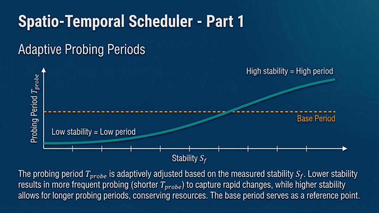
Lets look at how BRIGHT translates the policy decision into an actual probing schedule. Weve established that the contextual bandit selects a monitoring template, but that template only specifies a budget and base probing periods. The Spatio-Temporal Scheduler is responsible for the fine-grained allocation of those resources. This first part focuses on the temporal dimension: determining *when* to probe each flow. The core idea here is to dynamically adjust the probing period based on the flows stability. We start with the base probing period T_base, which is defined by the selected template and the flows category—remember, we classify flows into stable elephant, stable mouse, unstable, and event flows. We then use a proportional controller to adjust this period based on the flows stability score, S_f. If a flow is highly unstable, meaning its rate is fluctuating significantly, its stability score is low. This drives the probing period T_probe,f down, meaning we probe it more frequently. Conversely, a very stable flow gets a longer probing period, reducing overhead. This adaptive mechanism ensures that our limited monitoring budget is concentrated on the flows that are most difficult to estimate accurately, directly addressing the uncertainty quantified by the Bayesian model. This intelligent temporal allocation is critical for maximizing the accuracy we get from every single probe. Now we move to the second part of the scheduler: the spatial dimension.
|
 IEEE/ICACT20260358 Slide.11
[Big Slide]
[YouTube]