 |
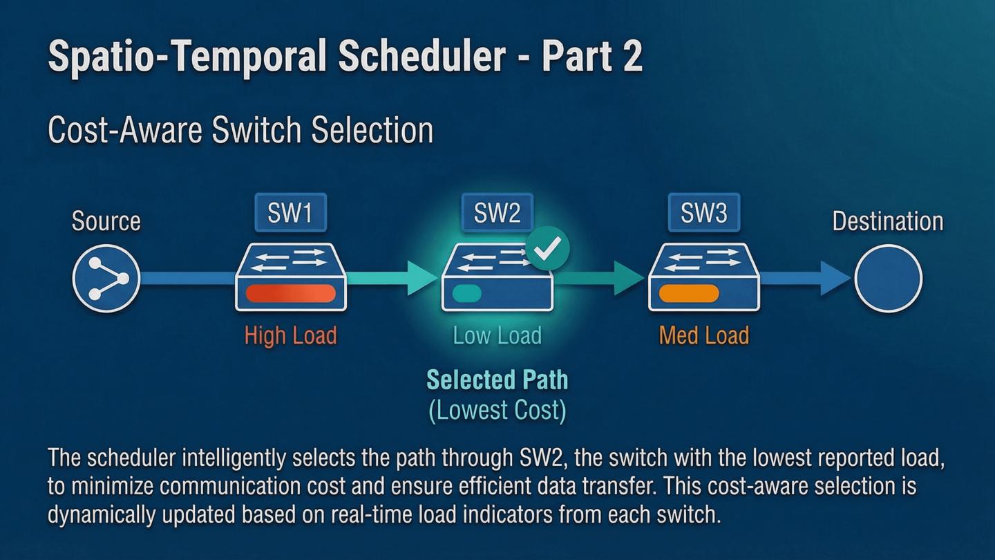
Having determined *when* to probe each flow, we now address the spatial dimension: *where* to probe it. This is a crucial optimization because polling different switches along a flows path incurs different costs and contributes differently to the overall load balancing. For every flow that needs to be probed in a given time slot, BRIGHT doesnt just pick the first switch. Instead, we consider all candidate switches along that flows path. We then select the switch that minimizes the total cost function. This cost function is designed to achieve two goals simultaneously: first, it minimizes the immediate cost of the query, and second, it ensures load balancing across all switches. By dynamically selecting the lowest-cost switch for each probe, we prevent any single switch from becoming a bottleneck due to excessive monitoring requests. This two-stage spatio-temporal approach—adjusting the probing frequency based on flow stability and selecting the polling switch based on cost and load—allows BRIGHT to achieve a fine-grained, highly efficient allocation of monitoring resources. This joint optimization is what truly sets our scheduler apart. With the scheduler detailed, lets put all these components together and see the main loop of the BRIGHT algorithm.
|
 IEEE/ICACT20260358 Slide.12
[Big Slide]
[YouTube]