Now 5212 visitors
Today:0 Yesterday:0
Total: 146322
215S 51P 5R
2026-10-21, Week 43 |
| Member Login |
| TACT Journal Homepage |
| Call for Paper |
| Committee |
| Find My Paper |
| Author Homepage |
| Statistics & History |
| Welcome Message |
| Paper Procedure |
| FAQ |
| Paper Archives |
| Outstanding Papers |
| Author Homepage |
| - Paper Procedure |
| - Journal Procedure |
| - Presentation Tips |
|
| Program & Proceedings |
| Program with Papers |
| Plenary Session |
| Tutorial Session |
|
| Presentation Platform |
| Hotel & Travel Info |
| About Korea |
| Accommodation |
| Transportation |
| VISA |
| Other Infomation |
|
| Photo Gallery |
| Scheduler Login |
| Seminar |
| Archives Login |
|
| Sponsors |

|

|

|

|

|

|

|

|

|

|
|
|
|
|
main_email:wxtdsg@mail.ustc.edu.cn
| Save the slide and description |

|
*** You can edit any slide by selecting the Slide number below***
|
 ICACT20230038 Slide.16
[Big slide for presentation]
[YouTube] |
Chrome Text-to-Speach Click!! |
 |
That's all. Thank you!
|
|
ICACT20230038 Slide.15
[Big slide for presentation]
[YouTube] |
Chrome Text-to-Speach Click!! |
 |
To summarize, we propose an efficient dynamic neural network for multispectral detection. Compared with the unoptimized static model, our proposed model reduces computation by 41% and off-chip memory access by 77% on.
We design a cross-layer scheduling for dynamic neural networks to improve the computation to communication (CTC) ratio. We designed the scheduling arbitration module, which can fine-tune fusion strategy according to the activation ratio of each layer at runtime to obtain the optimal scheduling scheme.
We implement a flexible FPGA-based hardware accelerator to evaluate our design. Experiments demonstrate that our dynamic neural network accelerator achieves a maximum 2.7× inference speedup.
|
|
ICACT20230038 Slide.14
[Big slide for presentation]
[YouTube] |
Chrome Text-to-Speach Click!! |
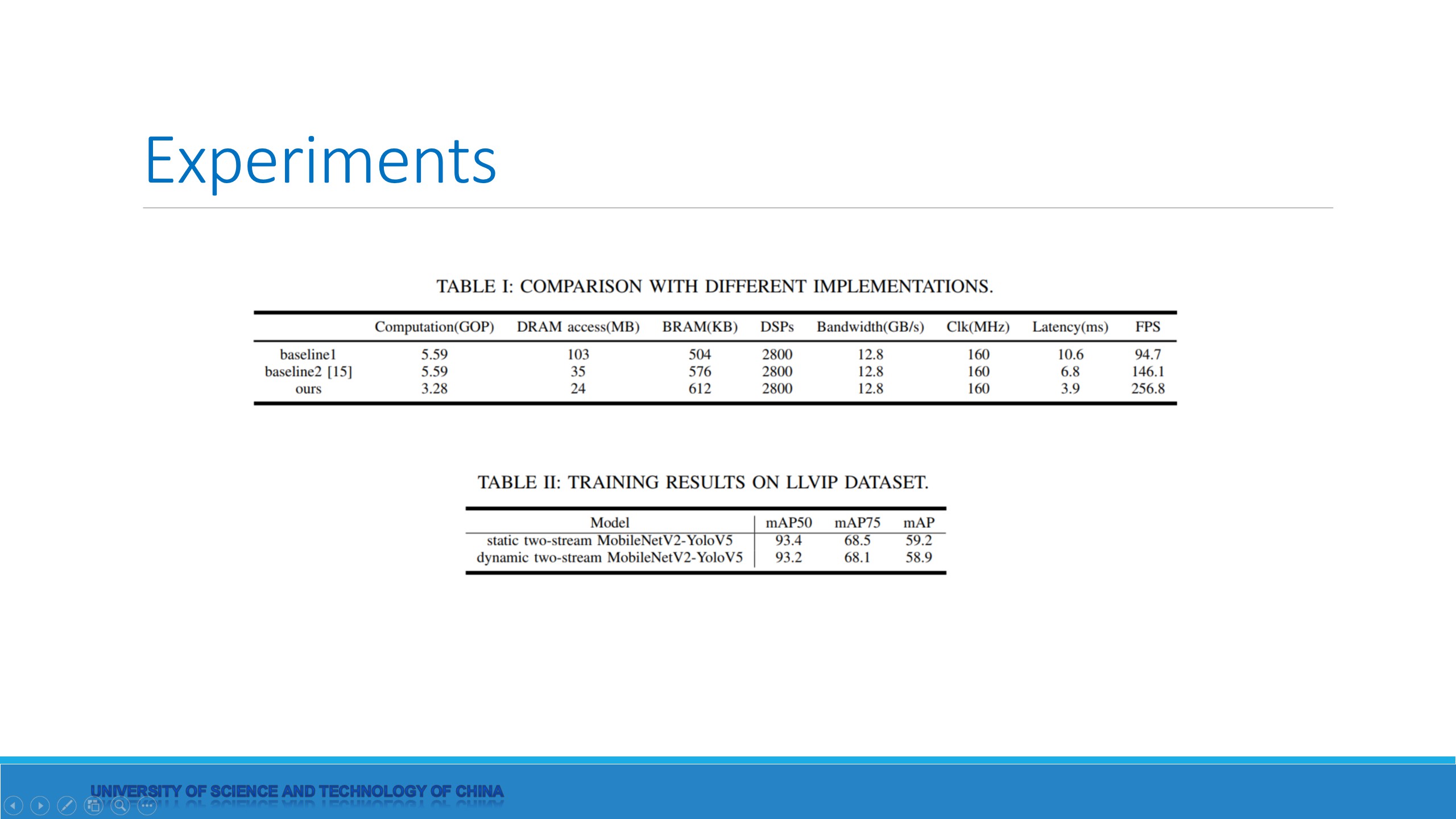 |
Table I shows the comparison with other baseline implementations. Benefiting from layers skipping and channel pruning, our dynamic neural network accelerator reduces the computational overhead by 41% and DRAM access by 77% compared to the unoptimized baseline1. Compared with baseline2, which only supports cross-layer scheduling for static networks, our implementation reduces the computational overhead by 41% and DRAM access by 31%. Therefore, the inference performance of our implementation is greatly improved by 1.8 -2.7times compared to the baseline.
Table 2 shows the training accuracy of dynamic and static networks on the multispectral detection dataset LLVIP. It can be seen that the accuracy of the dynamic network is close to the accuracy of the static network.
|
|
ICACT20230038 Slide.13
[Big slide for presentation]
[YouTube] |
Chrome Text-to-Speach Click!! |
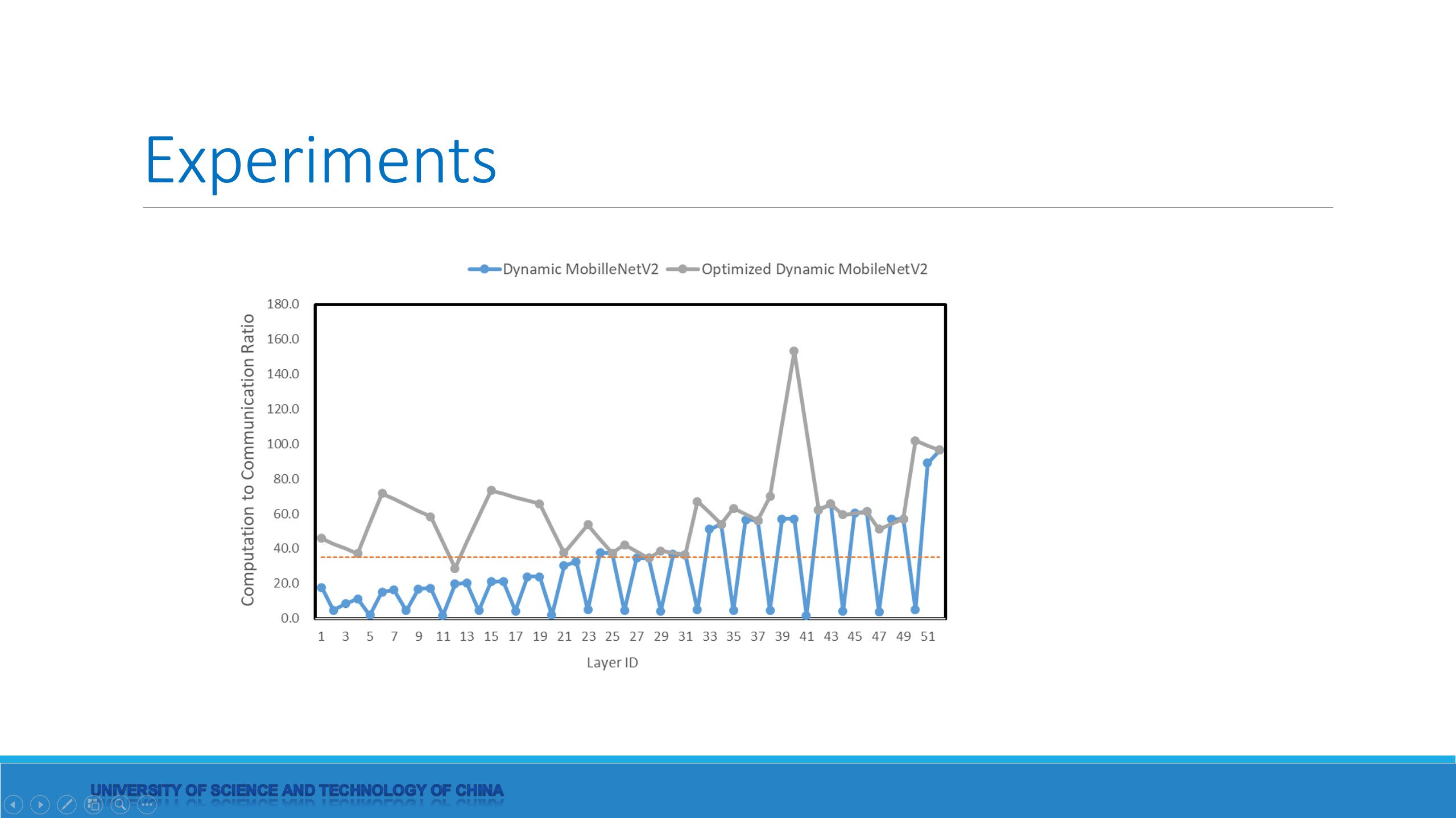 |
This figure shows the CTCs of the optimized dynamic neural network. After applying cross-layer scheduling, the CTCs of the optimized dynamic neural network are greatly improved, exceeding the threshold value C_0 of VC707. Therefore, the performance of the optimized model will not be limited by DRAM bandwidth, and DSP resources can be fully utilized.
|
|
ICACT20230038 Slide.12
[Big slide for presentation]
[YouTube] |
Chrome Text-to-Speach Click!! |
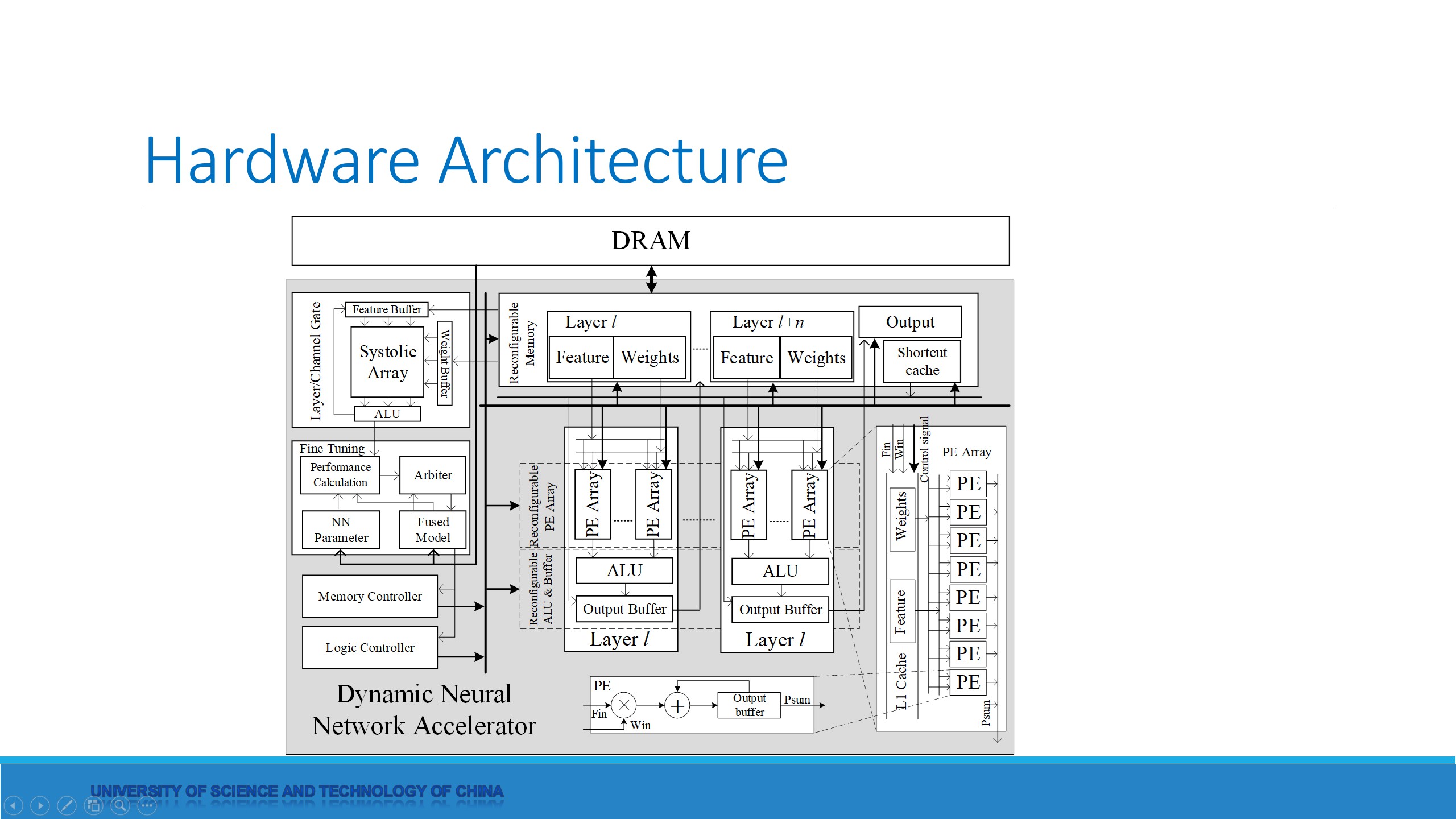 |
Layer/Channel Gate is a systolic array of size 10×10 used to perform MLP layers. Feature maps flow vertically and weights are accessed independently by the PEs. The results are accumulated in the local buffers and finally accumulated in each column. After the accumulation is completed, results are sent to the ALU unit for activation, quantization, and other operations. The activation information of layers and channels is sent to the fine-tuning module.
Fine-tuning module consists of four parts. Before processing the layers, the parameters of each layer of the network and the fused model are loaded from DRAM to the cache. The performance calculation module obtains the activation ratio of each layer at runtime, loads the network parameters and the fusion model, and then calculates the indicators such as CTC and off-chip memory access of the fine-tuned model. Since the search space is further limited, the amount of computation here is small and does not affect the overall performance. The search results are fed into the arbiter, which selects the optimal model and updates the fused model cache.
To adapt to different cross-layer scheduling strategies, we introduce a reconfigurable processing module composed of fine-grained PE arrays, ALUs, and buffers. Each PE array consists of 8 PEs. The PEs in the PE array are cascaded to each other. Data flow can be transmitted and broadcast among the PE arrays and PEs for data reuse.
All the configurable units are divided into multilayers. The division is according to the proportion of the computational cost of different layers so that the throughput of different layers is balanced. With the appropriate division, the intermediate data can be consumed by the next layer in time. When the processing module starts working, the PE arrays read the features and weights from the SRAM and share them with different PEs.
PEs produce the partial sums and pass them to the Arithmetic Logic Units (ALUs). The partial sums are accumulated in the ALUs. After the accumulation of partial sums is completed, the ALUs will re-quantize the output data from 32-bit to 8-bit. Then the output will be cached in the output buffer and passed to the next layer.
|
|
ICACT20230038 Slide.11
[Big slide for presentation]
[YouTube] |
Chrome Text-to-Speach Click!! |
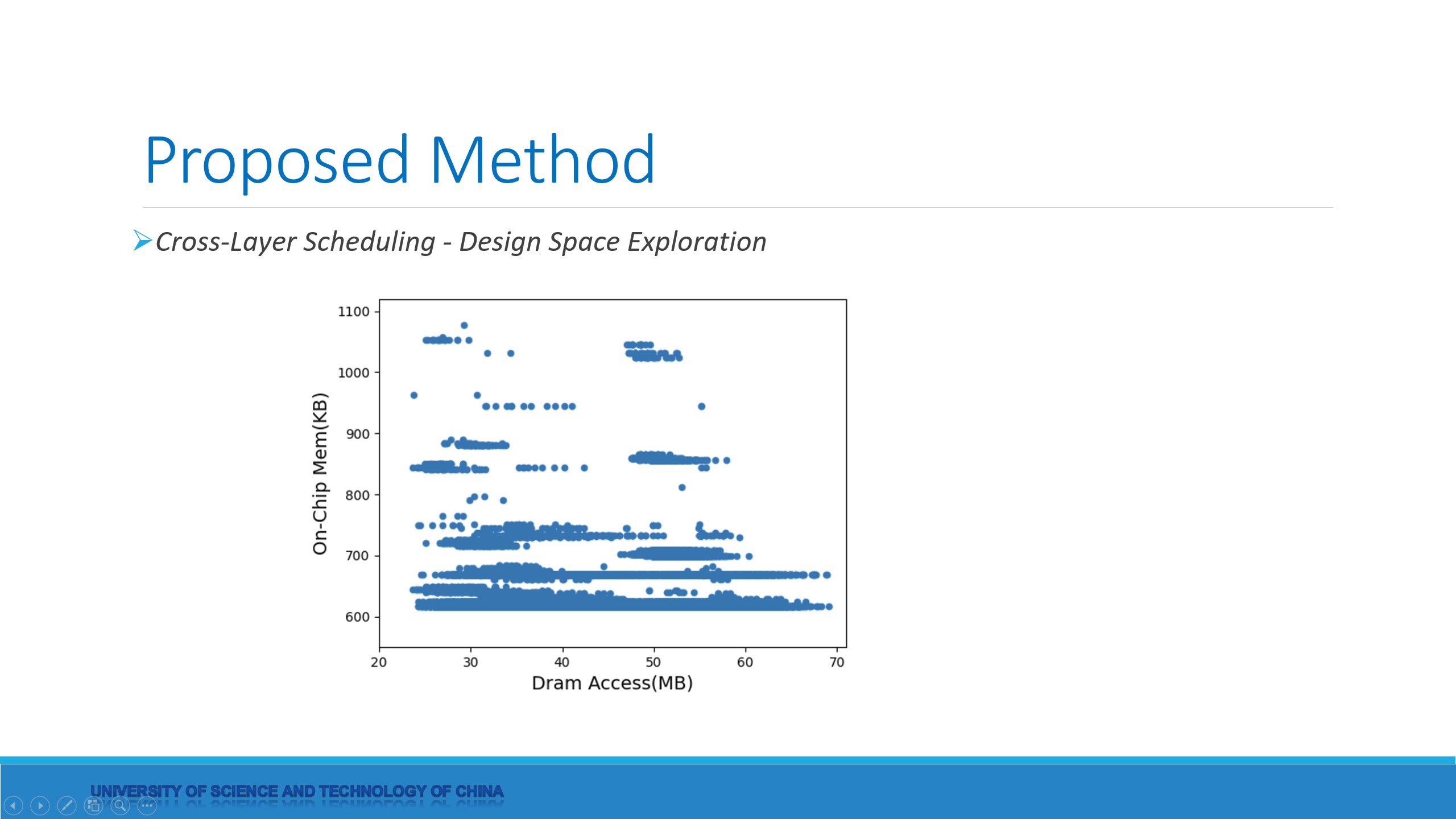 |
In the collection, the size of on-chip memory and the DRAM access is different, depending on the structure of these models. A scatter plot can be drawn, as shown in figure. Among them, the relatively good implementation in both indicators is selected as the final fusion model.
During the inference, the activation ratio of each layer may fluctuate, which affects the performance of the cross-layer scheduling. So we design a fine-tuning module in the accelerator. The fusion strategy is fine-tuned based on the actual activation ratio computed at runtime. The fine-tuning algorithm limits the search space and only fine-tunes 2 layers at most, so the computational overhead is minimal. The arbiter can judge the fine-tuned model, and select the fusion model with the best performance to replace the previous model.
|
|
ICACT20230038 Slide.10
[Big slide for presentation]
[YouTube] |
Chrome Text-to-Speach Click!! |
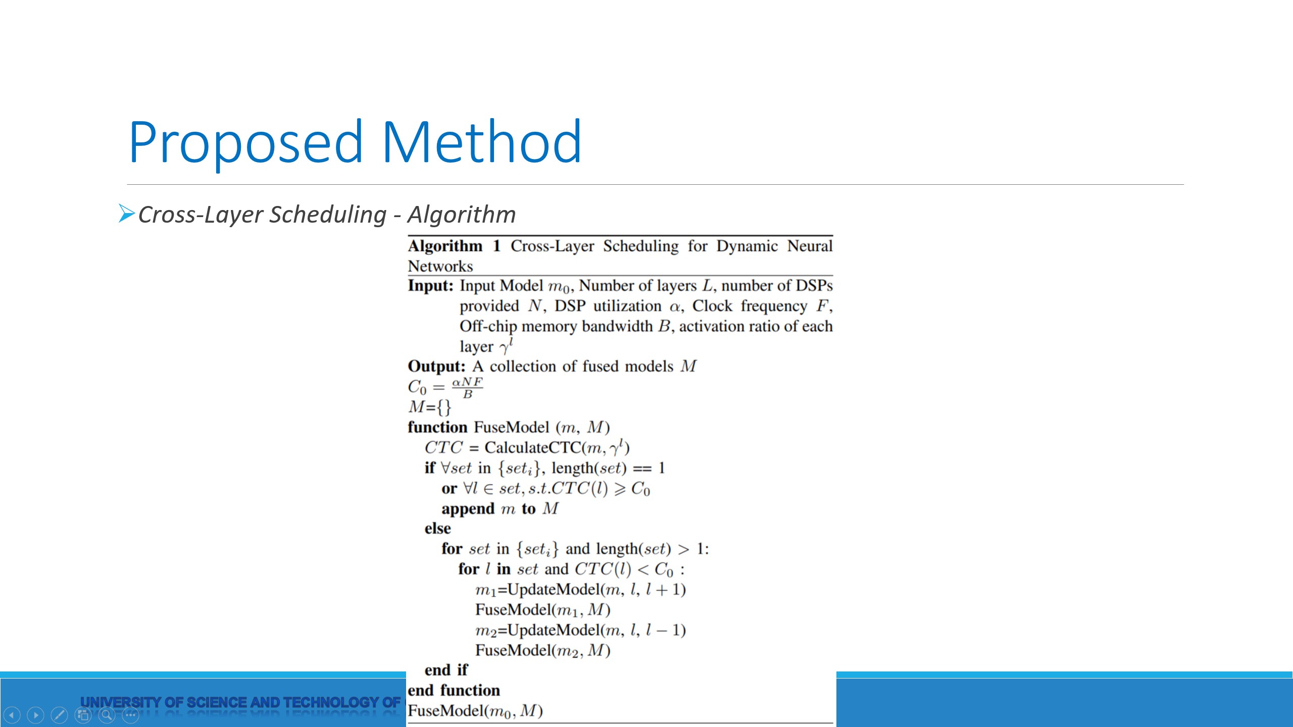 |
Algorithm illustrates the design space exploration for cross-layer scheduling of dynamic networks. First, we calculate the threshold C_0. Then, according to the model m and the activation ratio γl., the theoretical CTC value of each layer can be calculated. In any subset which consists of at least two convolutional layers, an arbitrary layer with CTC less than C_0 is selected and fused with the previous or next layer to get the fused model m. Then the fused model is sent to the next iteration and the above operation is repeated. When either of the following two conditions is met, 1) all the convolutional layers in one subset are fused; 2) the theoretical CTCs of all layers are greater than the threshold C_0, we terminate the iteration and obtain a fusion model m. Repeat the exploration and try different fusion branches. After traversing all the search spaces, we can get a collection M.
|
|
ICACT20230038 Slide.09
[Big slide for presentation]
[YouTube] |
Chrome Text-to-Speach Click!! |
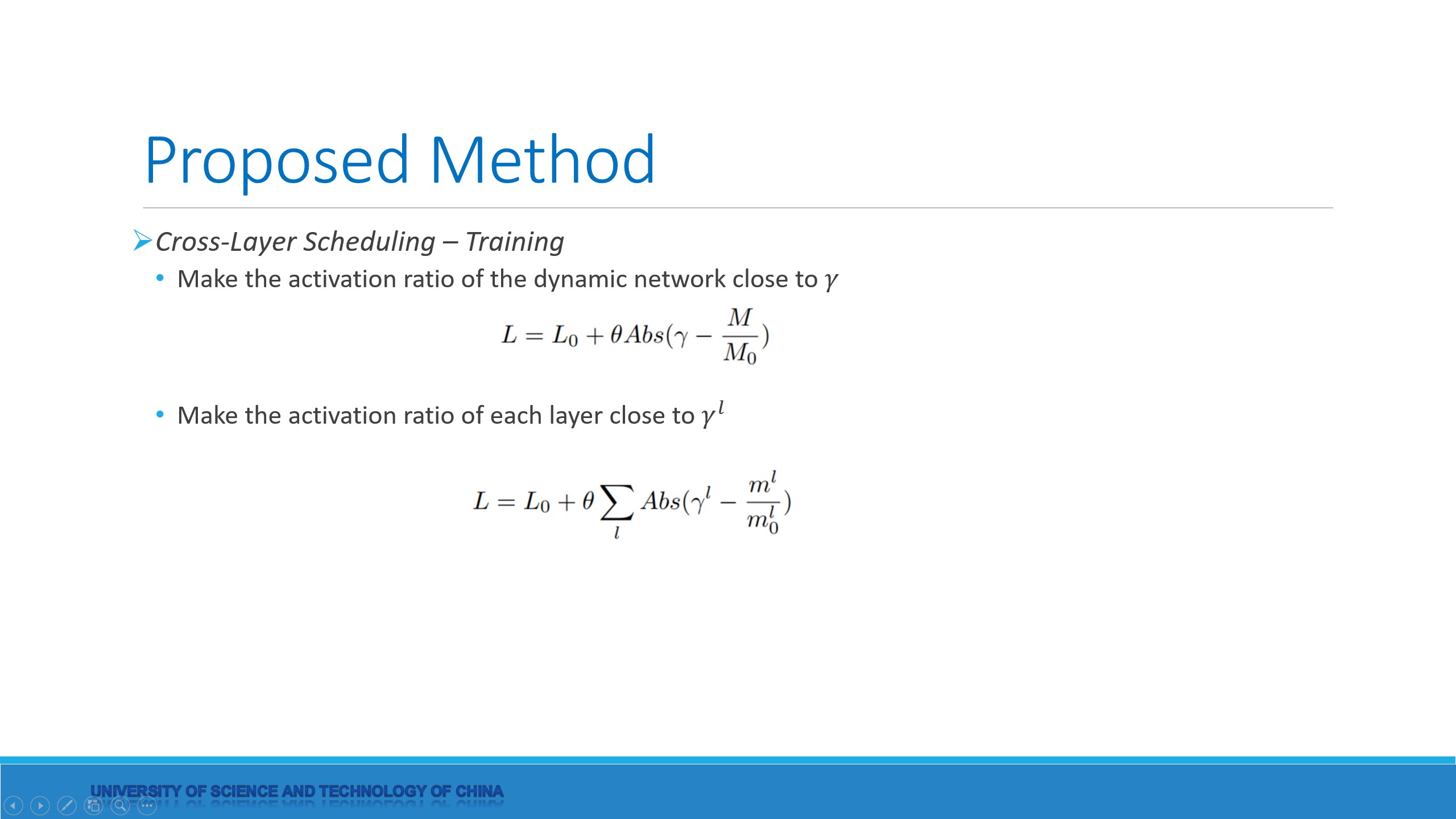 |
As the conventional dynamic neural network processes different samples, its network structures are very different, so it is difficult to make a static analysis and determine the fusion strategy. To facilitate analysis, we set the model activation ratio to γ. The total computation of the static network is recorded as M_0, and the computation of each layer is recorded as m^l_0. In the training phase, we count the actual computation of each sample after layer skipping and dynamic pruning, which is recorded as M, and the actual computation of each layer is recorded as m^l. We divided the training into two steps. In the first step, we add a new item to the loss function:
where θ is a configurable parameter. We train the model until convergence and then obtain weights that make the overall activation ratio of the dynamic network close to γ. In the second step, we select a batch of samples for inference, count the actual activation ratio of each layer, and average them. Then we obtain the average activation ratio of each layer γl. The loss function is modified as follows. We train the model again. Finally, while ensuring accuracy, the activation ratio of each layer is close to the fixed value γl.
|
|
ICACT20230038 Slide.08
[Big slide for presentation]
[YouTube] |
Chrome Text-to-Speach Click!! |
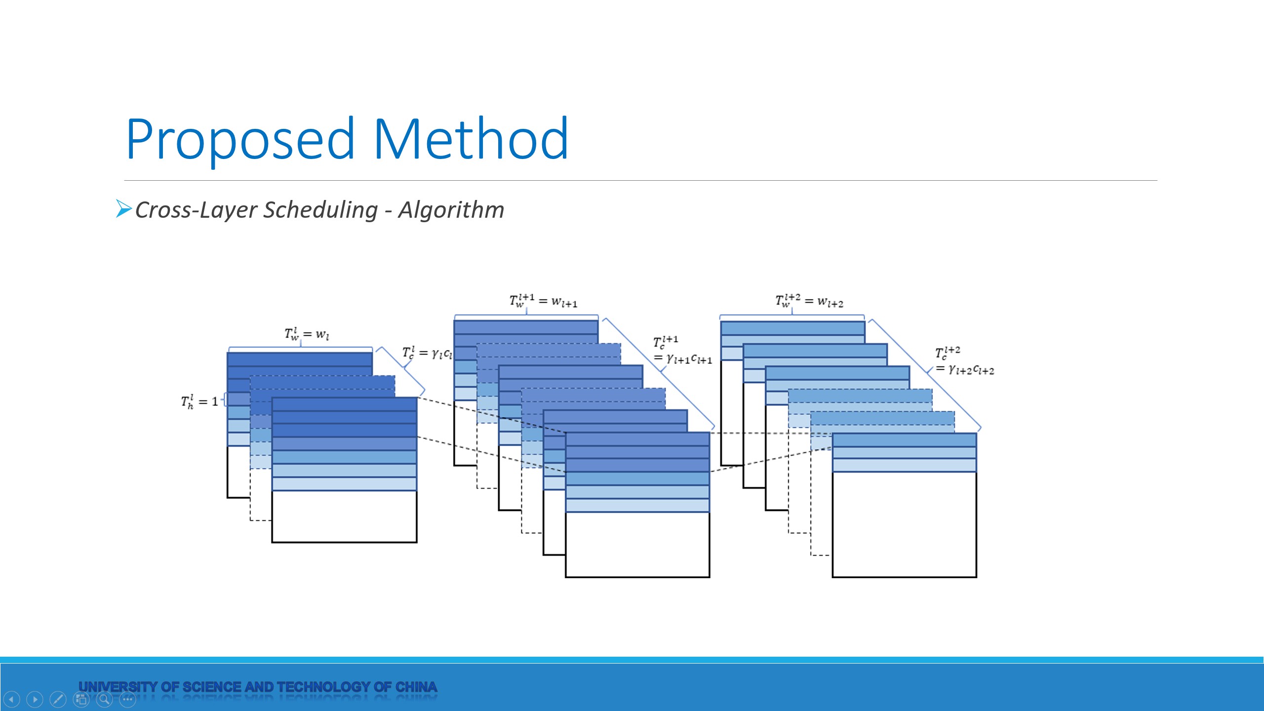 |
In convolutional layers, the output pixel correlates with part of the input pixels. So we can get the output pixel directly without computing all the intermediate features. We propose the cross-layer scheduling for dynamic neural networks, so that the off-chip memory access of intermediate layers can be reduced and CTC can be improved.
This figure illustrates the cross-layer scheduling of two convolutional layers, and the kernel sizes are 1 times 1 and 3 times 3. The dashed lines represent the pruned channels. Data has to be tiled due to limited on-chip memory, and T_h, T_w, T_c denote the tile shape of height, width, and channels, respectively. If the data is tiled on C dimension, then extra partial sums will be produced, resulting in 4 times memory overhead (the features are 8-bit quantized and partial sums are 32-bit). In order to benefit the DMA transactions with continuous data, we cache the entire row in the on-chip SRAM. Therefore, it is more appropriate to tile on H dimension.
|
|
ICACT20230038 Slide.07
[Big slide for presentation]
[YouTube] |
Chrome Text-to-Speach Click!! |
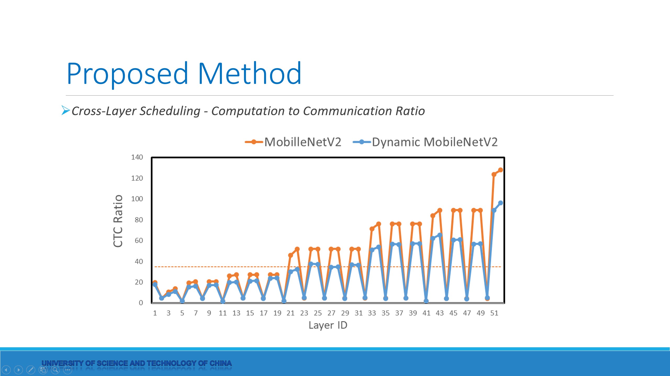 |
Since it is not known in advance which channels will be activated, all input channels will inevitably be loaded. With the reduction of computation, the CTC of the convolutional layer decreases further. This figure statistically shows the theoretical CTC values of each layer in the static network and the dynamic network. It can be seen that the system is memory-bounded.
|
|
ICACT20230038 Slide.06
[Big slide for presentation]
[YouTube] |
Chrome Text-to-Speach Click!! |
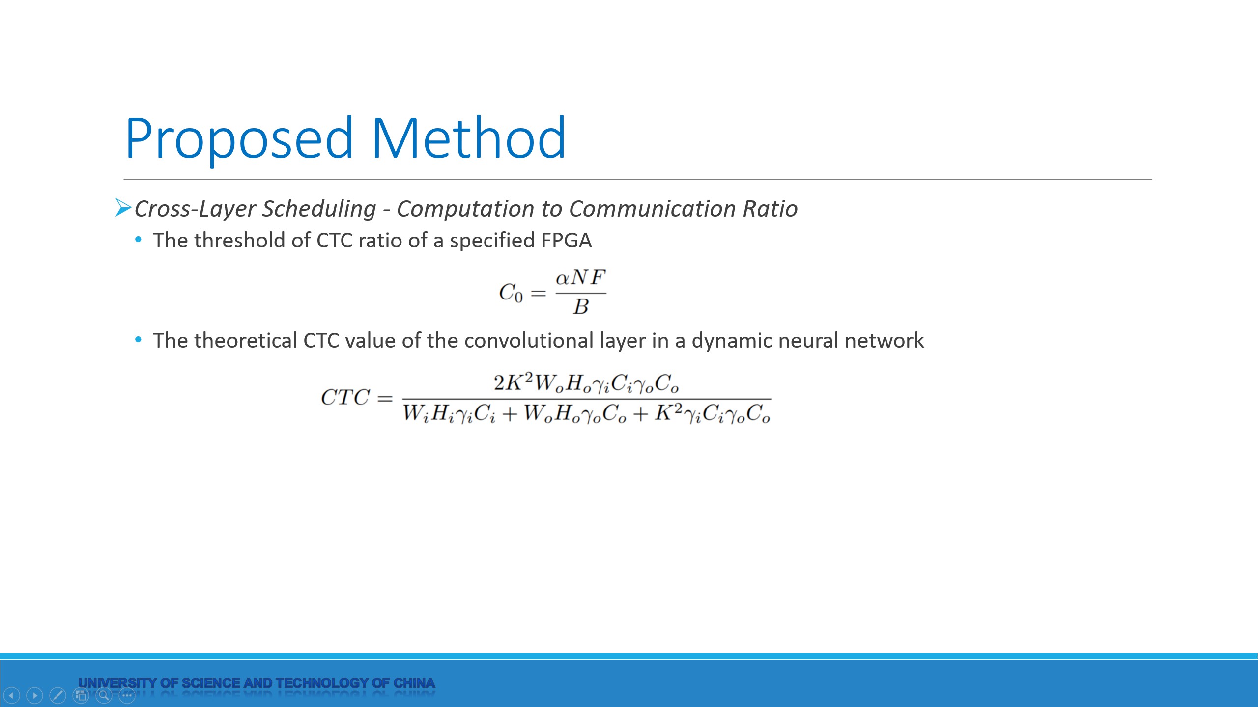 |
Computing and communication are two key constraints limiting system throughput. Computation to communication ratio features the number of operations performed per memory access. A high CTC indicates that the layer is computationally intensive, and the inference latency is determined by the number of computational resources. On the contrary, a low CTC means the off-chip bandwidth greatly affects the performance
The threshold of CTC ratio C_0 of a specified FPGA can be calculated by this formulation. N is the number of DSP slices provided by the FPGA, α is the utilization of DSPs. F is the clock frequency, and B is the off-chip memory bandwidth.
The theoretical CTC value of the convolutional layer in a dynamic neural network can be calculated by this formulation. Where W and H denote the width and height, C denotes the number of channels, K denotes the kernel size and γ denotes the activation ratio of channels at the current layer. The subscripts i and o represent the input and output feature maps, respectively.
|
|
ICACT20230038 Slide.05
[Big slide for presentation]
[YouTube] |
Chrome Text-to-Speach Click!! |
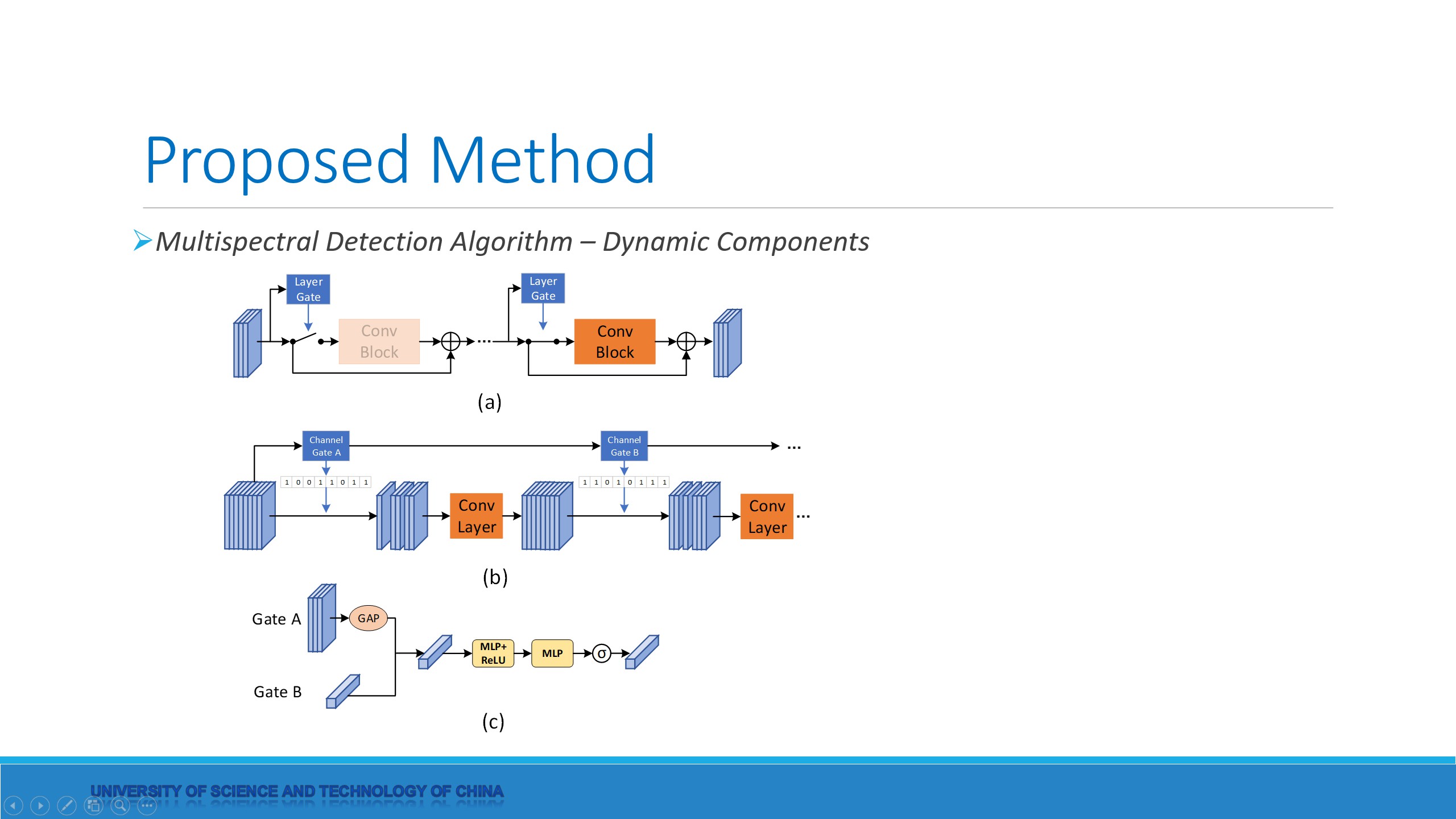 |
On this basis, we take two dynamic components: 1) Layer skipping; 2) Dynamic pruning. Each stage contains multiple convolutional blocks, and the layer skipping module is embedded before each stage. The layer gate generates 1-bit data according to the input of the convolution block, and determines whether to skip the current convolution block. Dynamic pruning is used before convolutional layers. The Channel gate is embedded before the convolutional layer. According to the input, several bits of data are generated to determine whether each channel will be pruned. The layer gate and channel gate use Global Average Pooling (GAP) for dimensionality reduction. After two MLPs, the hard-sigmoid function is used to restrict the vector's range to (0,1). Finally, the vector is binary quantized to 0 or 1.
In dynamic pruning, there are many ways to generate channel weights. Some works generate the weights taking the feature maps of each layer as the input. Some builds an additional decision network and take the input picture as input. We take a mixed approach. The input feature is sent to channel gate A, which is located before the first layer of one or several convolutional blocks. Gate B takes the output of the previous gate as its input. The network is divided into multiple subsets by channel gate A.
|
|
ICACT20230038 Slide.04
[Big slide for presentation]
[YouTube] |
Chrome Text-to-Speach Click!! |
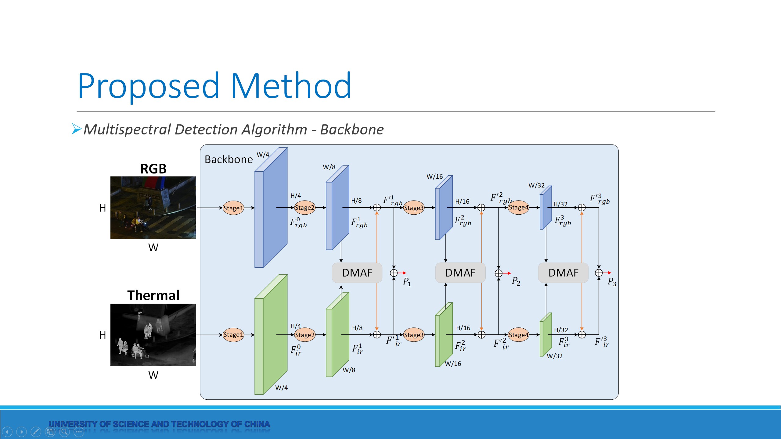 |
We propose a dynamic neural network for multispectral detection, as shown in the picture. It is a two-stream model extended from Yolov5. The backbone is replaced by the lightweight MobileNetV2, in which the fusion module adopts Differential Modality Aware Fusion Module (DMAF) proposed by MBNet.
|
|
ICACT20230038 Slide.03
[Big slide for presentation]
[YouTube] |
Chrome Text-to-Speach Click!! |
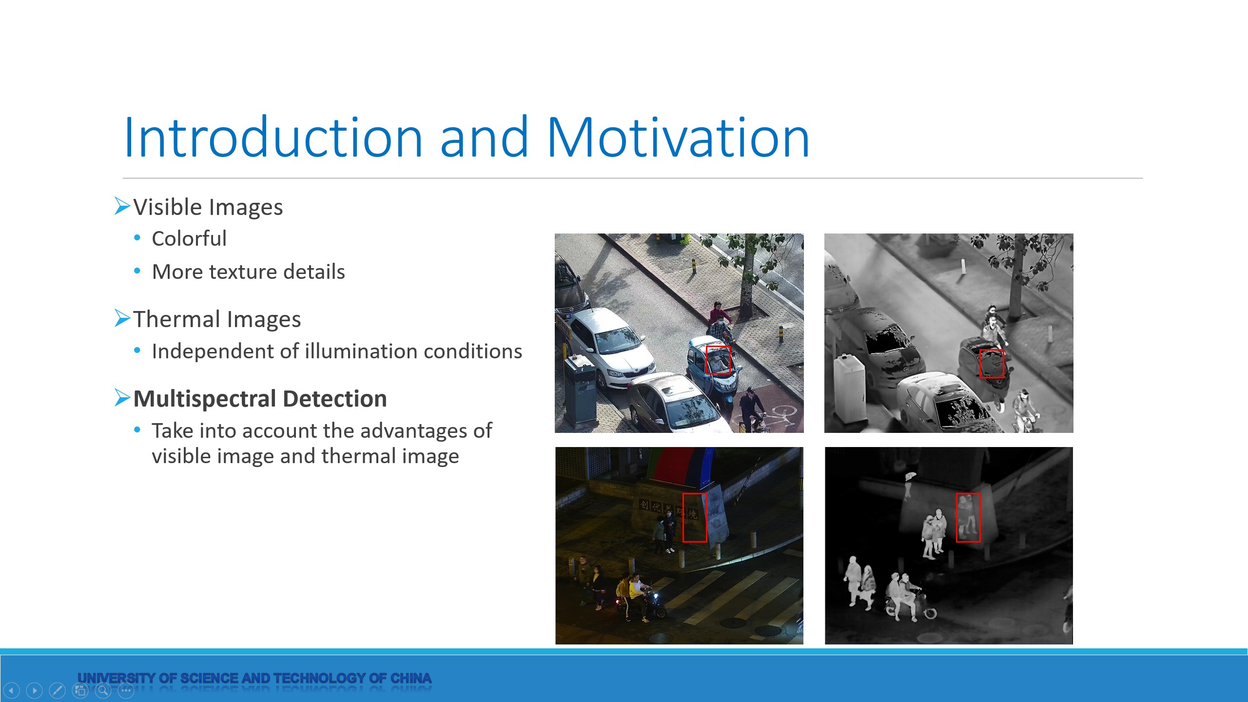 |
Visible images are colorful and have more texture details. Thermal images lose the information. Thermal images can be imaged clearly in dark scenes, because the image quality is independent of the illumination condition. As visible and thermal images have their own advantages and disadvantages in different scenarios, researchers have raised interest in multispectral detection.
In many application scenarios, such as autonomous driving, high accuracy and low latency are required for multispectral detection. At the same time, it is desired to reduce cost, chip area, and power consumption as much as possible. However, to ensure accuracy, multispectral detection commonly uses a two-stream architecture. Compared with the traditional CNN model, it requires more computational resources, more on-chip memory, and higher off-chip bandwidth. To address this problem, using dynamic neural networks is a feasible solution. Compared to static neural networks, dynamic networks selectively activate model components based on the input sample during inference. Studies have shown that dynamic neural networks have greater computational efficiency and representation capability.
It is challenging to process dynamic neural networks efficiently, due to the significant irregularities introduced by the redundancy elimination at runtime. General hardware accelerators are difficult to benefit from dynamic architectures, because they can not efficiently process optimized models, and eliminate redundant computing and memory access.
|
|
ICACT20230038 Slide.02
[Big slide for presentation]
[YouTube] |
Chrome Text-to-Speach Click!! |
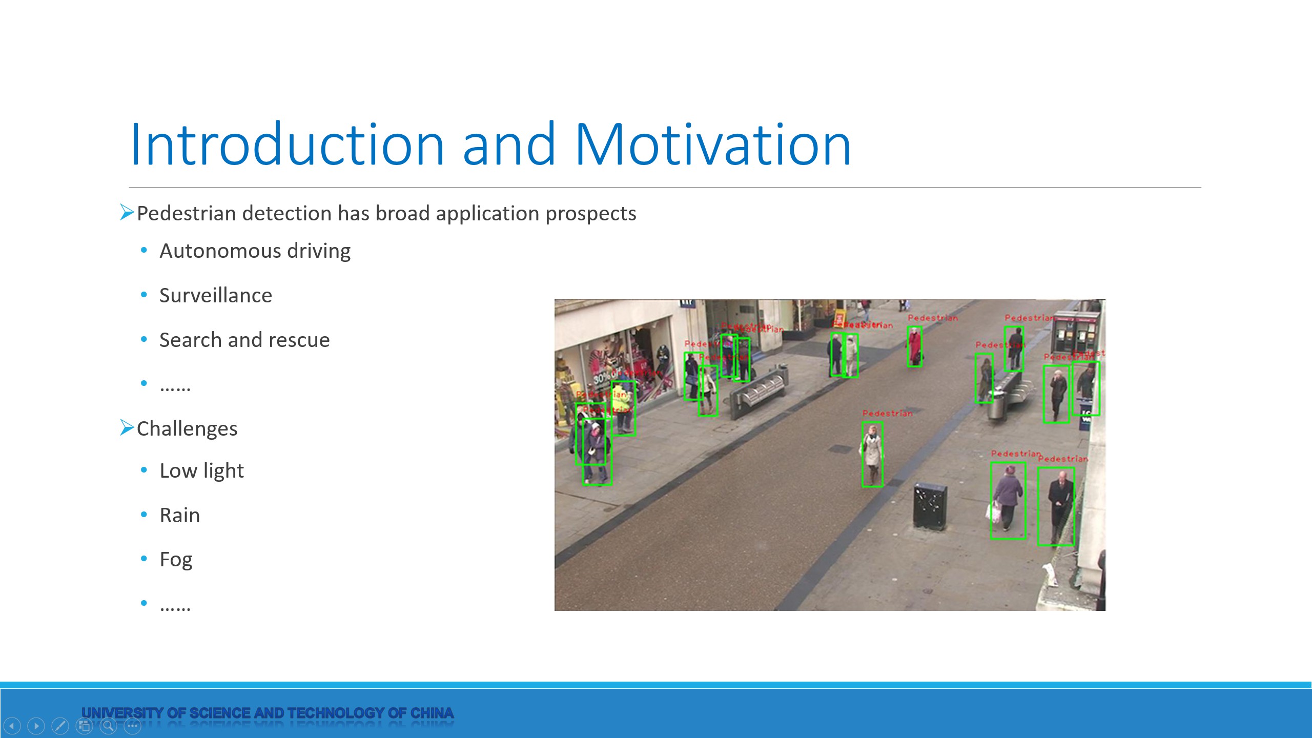 |
Pedestrian detection is a classic and important computer vision task, and it has broad application prospects, such as autonomous driving, surveillance, search and rescue and so on. However, in real-world applications, the environment is often complex and changeable, such as low light, rain, fog. In these cases, pedestrian detectors that only focus on a single sensor may have difficulty achieving high accuracy.
|
|
ICACT20230038 Slide.01
[Big slide for presentation]
[YouTube] |
Chrome Text-to-Speach Click!! |
 |
Hello, everyone. The topic of our work is ‘Dynamic Neural Network Accelerator for Multispectral detection Based on FPGA’.
|
| |