ICACT20210223 Slide.18
[Big slide for presentation] |
Chrome Text-to-Speach Click!! |
 |
Thank you for your listening. Your comments or questions are very welcomed.
|
|
ICACT20210223 Slide.17
[Big slide for presentation]
|
Chrome Text-to-Speach Click!! |
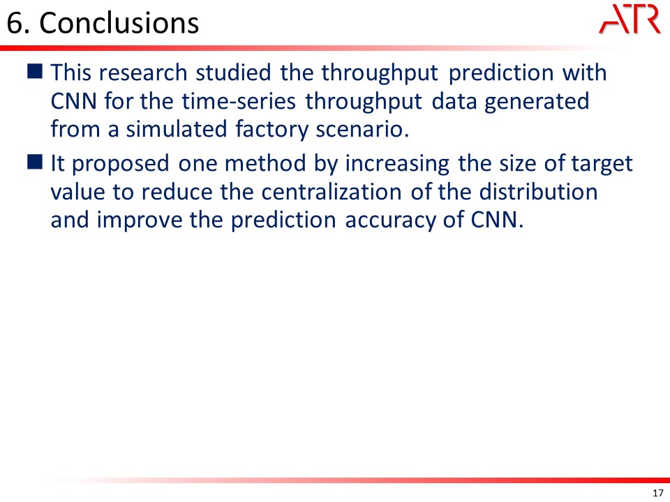 |
This research studied the throughput prediction with CNN for the time-series throughput data generated from a simulated factory scenario. It proposed one method by increasing the size of target value to reduce the centralization of the distribution and improve the prediction accuracy of CNN.
|
|
ICACT20210223 Slide.16
[Big slide for presentation]
|
Chrome Text-to-Speach Click!! |
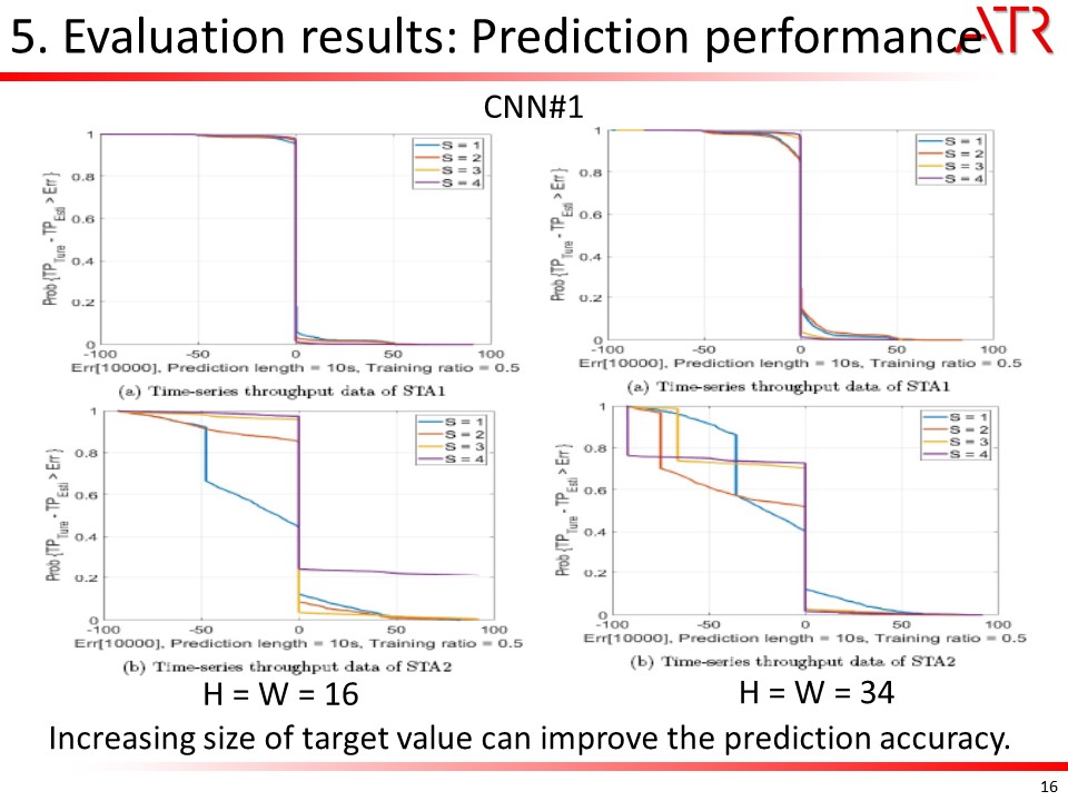 |
These figures show the prediction performance of CNN#1 using the proposed target vectorization where the sizes of input matrix are (H=W=16) and (H=W=34), respectively. The parameters of CNN#1 and calculation process are the same with the previous section. From the figures we can confirm that the prediction accuracy is improved for both the throughput data from STA1 and STA2.
|
|
ICACT20210223 Slide.15
[Big slide for presentation]
|
Chrome Text-to-Speach Click!! |
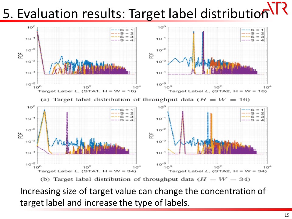 |
This figure shows the target label (L) distribution of throughput data of both STAs for different sizes of the input matrix. The size of target vector S is changed from 1 to 4. It is shown that the distribution of label after target vectorization is spread over a wider range as S is increased. More labels appear which makes the CNN have more options for its input. Therefore, it benefits the improvement of prediction accuracy.
|
|
ICACT20210223 Slide.14
[Big slide for presentation]
|
Chrome Text-to-Speach Click!! |
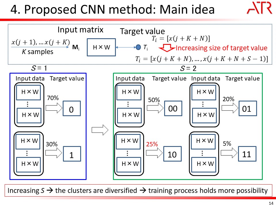 |
One efficient way to reduce such prediction loss is to make vectorization of target or increase the length of target. This figure shows the proposed idea. Suppose an on-off time-series data has two values as on (1) with 70% and off (0) with 30%, respectively. For the ith input matrix M_i of the conventional CNN, the target is usually a scalar (0 or 1) as T_i. Therefore, the training process finds the weight to make the predicted results as 1 or 0 with 70% or 30%, respectively. Therefore, even if some rare input matrices appear, the predicted values are also judged as 1 or 0 with 70% or 30%, respectively. Different with a single target, target vectorization can make the target value is not a scalar but a vector as. With this simple process, it can improve the prediction accuracy for the occurrence of some rare input matrices. From this figure, two consecutive data are used as one target for each input matrix. In such case, the target vector can be four candidates with different probabilities. This process makes the distribution more even than that of (S = 1).
|
|
ICACT20210223 Slide.13
[Big slide for presentation]
|
Chrome Text-to-Speach Click!! |
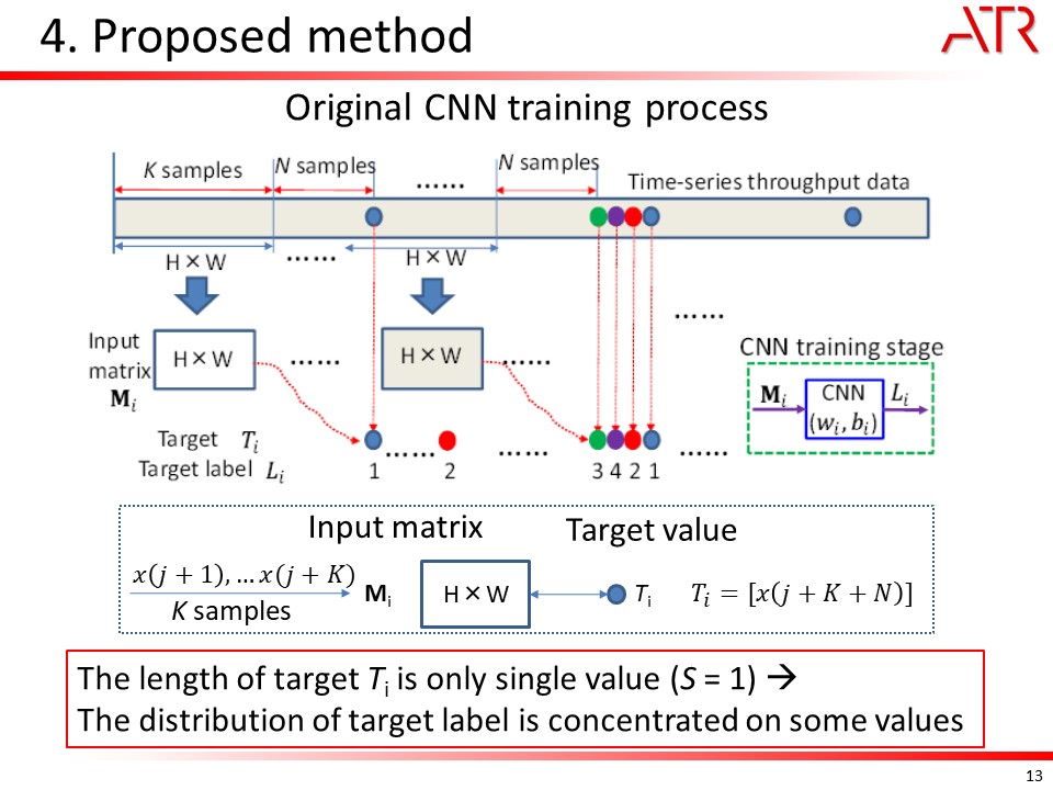 |
The CNN can obtain promising performance especially when the targets of input data or image have an even distribution. However, when target includes a few values which occupy major distribution, the prediction process is apt to make the predicted value near to these values after training process. Therefore, some rare values are neglected which may reduce the prediction accuracy.
|
|
ICACT20210223 Slide.12
[Big slide for presentation]
|
Chrome Text-to-Speach Click!! |
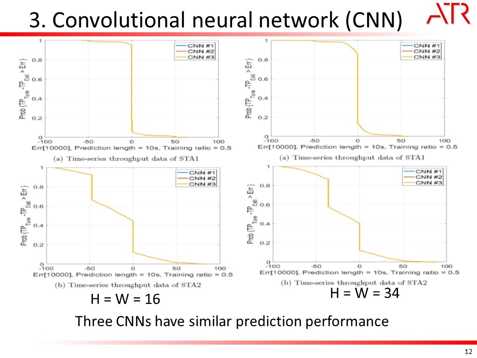 |
The complementary cumulative distribution function (CCDF) of the prediction error of throughput data using three CNNs are shown in left figure with (H=W=16) and right Figure with (H=W=34), respectively. All the three CNNs have almost identical prediction accuracy. The results imply that the throughput data from both STAs are all simple. Therefore, the simplest structure of CNN (CNN\#1) is enough to fully capture the feature of time-series throughput data. On the other hand, the results imply that using a small size of input matrix can further capture the data pattern for CNNs.
|
|
ICACT20210223 Slide.11
[Big slide for presentation]
|
Chrome Text-to-Speach Click!! |
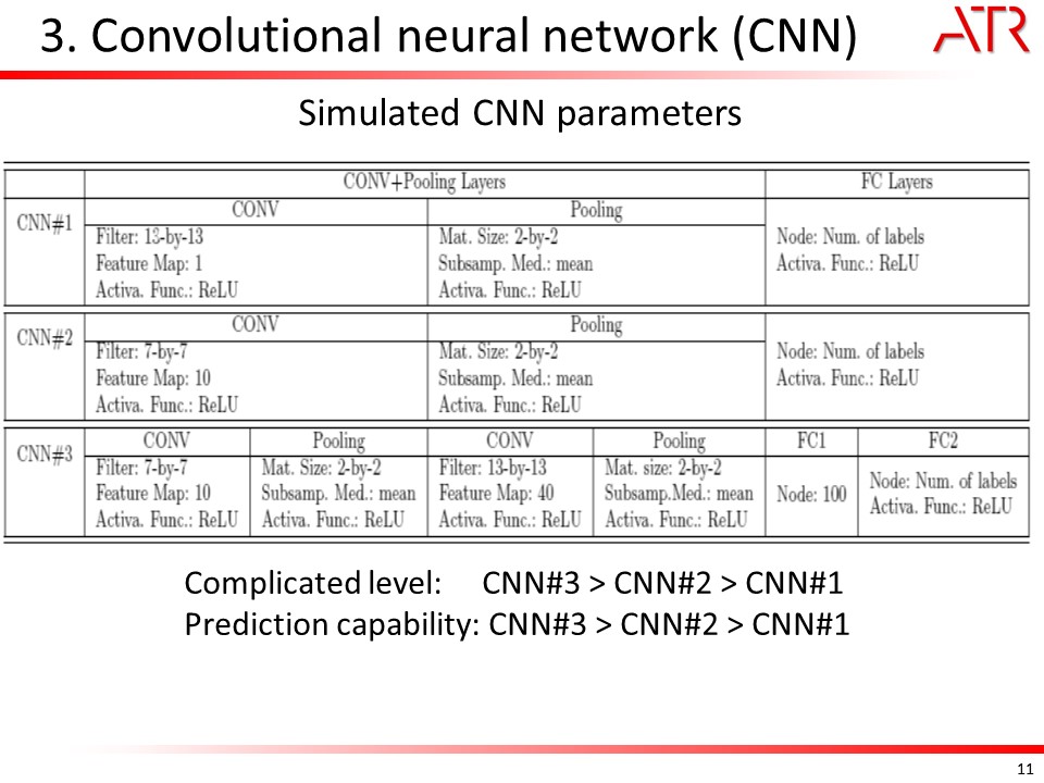 |
We designed three kinds of CNN for throughput prediction which called CNN1, CNN2 and CNN3. The parameters of each CNN are given in this table. The complexity of these CNNs is like CNN3>CNN2>CNN1 which is similar to the prediction capability.
|
|
ICACT20210223 Slide.10
[Big slide for presentation]
|
Chrome Text-to-Speach Click!! |
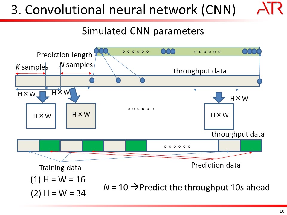 |
Here we simulated CNN with the parameters as follows, the filter size H and W is selected as 16 and 34. The prediction length is set as 10 seconds which means that the throughput data is predicted for the 10s ahead. The training data and prediction data is employed as this figure. We use half data for training and the left half for prediction.
|
|
ICACT20210223 Slide.09
[Big slide for presentation]
|
Chrome Text-to-Speach Click!! |
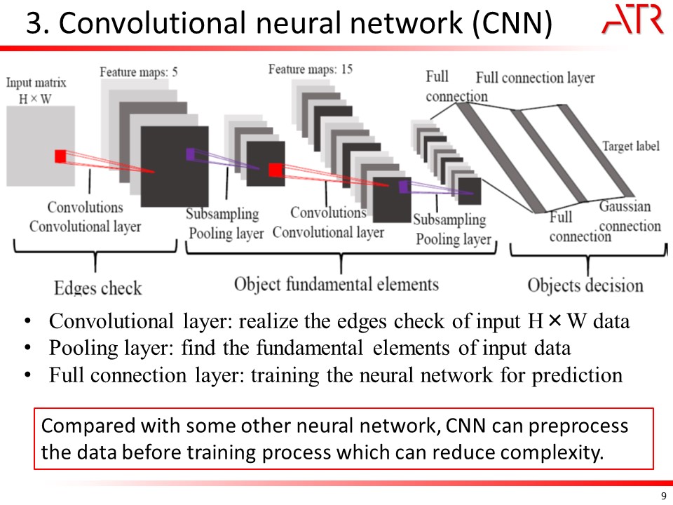 |
Let me give a simple explanation on the fundamental structure of CNN and the related functions. Generally, CNN includes three major layers: convolutional layer, pooling layer and fully-connected layer. The convolutional layer computes the output of neurons that are connected to local regions in the input matrix. All neurons compute a dot product between their weights and a small region through which they are connected to the input matrix. Such local regions can be defined as a filter with small width and height to reduce the computational complexity. The output of each filter is called a ``feature map'' which shows the effect of an edge check. Then the pooling layer performs a down-sampling operation along the spatial dimensions and places the data in a small volume. CNN can have several convolutional layers and pooling layers to dig the fundamental elements of image data. Finally, the fully-connected (FC) layer combines all fundamental elements of image data to provide the final decision.
|
|
ICACT20210223 Slide.08
[Big slide for presentation]
|
Chrome Text-to-Speach Click!! |
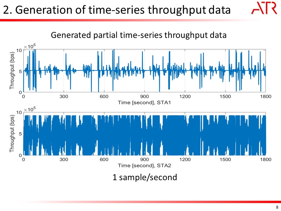 |
The throughput is calculated using the generated MCS value from the ray-trace model in each second. We have generated 8-hour theoretical throughput data and the 30-min theoretical throughput of both links are shown in this figure. The throughput of both links varies according with time. The reason is that the moving route error will make the RSS different even if the route is planned as 45m each side. The different RSSI changes the throughput between two links, and it becomes more unpredictable.
|
|
ICACT20210223 Slide.07
[Big slide for presentation]
|
Chrome Text-to-Speach Click!! |
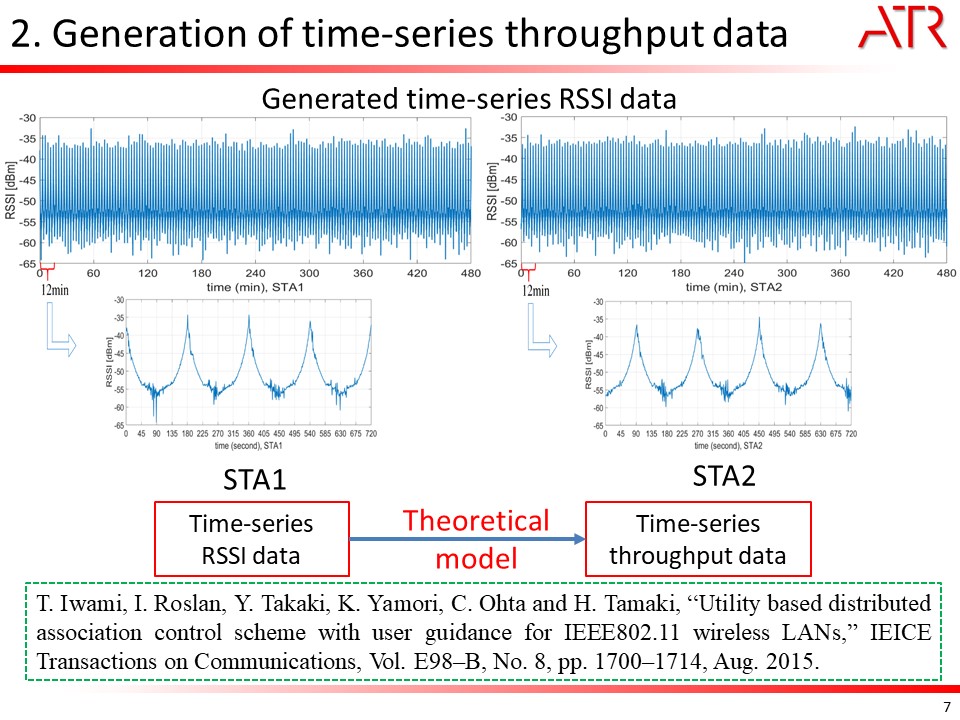 |
The generated time-series RSSI data of two STAs are given in these figures. From 12min RSSI waveform, we can find the RSSI data has some periodic pattern because each STA moves with fixed route. But due to route error, some RSSI has different value for the same location. After obtained time-series RSSI data, we use a theoretical model to calculate the time-series throughput data according to the following reference. we assume that both STA1 and STA2 have cameras which face different directions and each camera requires 510~kbps throughput at STA1 and 760~kbps throughput at STA2 for video transmission, respectively.
|
|
ICACT20210223 Slide.06
[Big slide for presentation]
|
Chrome Text-to-Speach Click!! |
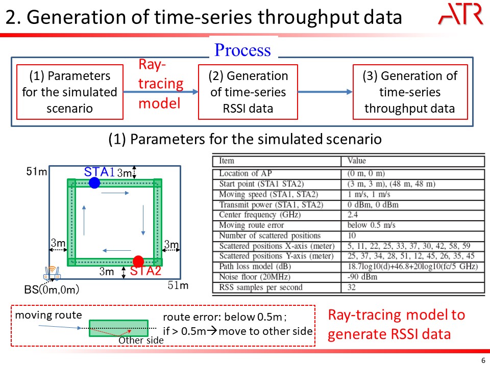 |
Let us explain how to get the throughput data considering the simple factory environment. We first simulated a 51m-by-51m factory scenarios with two moving STAs. Two moving STAs with high resolution cameras as monitors which capture the real-time data to send the AP side. The moving routes for both STAs are clockwise with speed as 1m/s. The distance between two STAs is about 90m. The moving route also includes route error within about ±0.25m. When moving STA deviates the main route to ±0.25m, the moving direction will be changed to other side. The simulation parameters are listed in Table. We selected ray-trace channel model to get the channel variation and then RSSI values. The simulation utilizes 10 constant scattered positions to generate the reflected paths at each location of STA1 and STA2. The channel response and then RSSI value are calculated using the distances of reflected paths and LOS path.
|
|
ICACT20210223 Slide.05
[Big slide for presentation]
|
Chrome Text-to-Speach Click!! |
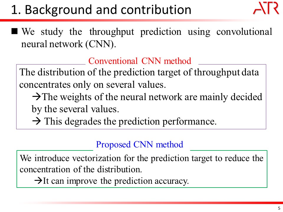 |
In this paper, we will study the throughput prediction using convolutional neural network (CNN). For conventional CNN, the distribution of the prediction target of throughput data concentrates only on several values. Therefore, the weights of the neural network are mainly decided by the several values which degrades the prediction performance. To solve this issue, we introduce vectorization for the prediction target to reduce the concentration of the distribution, which can improve the prediction accuracy.
|
|
ICACT20210223 Slide.04
[Big slide for presentation]
|
Chrome Text-to-Speach Click!! |
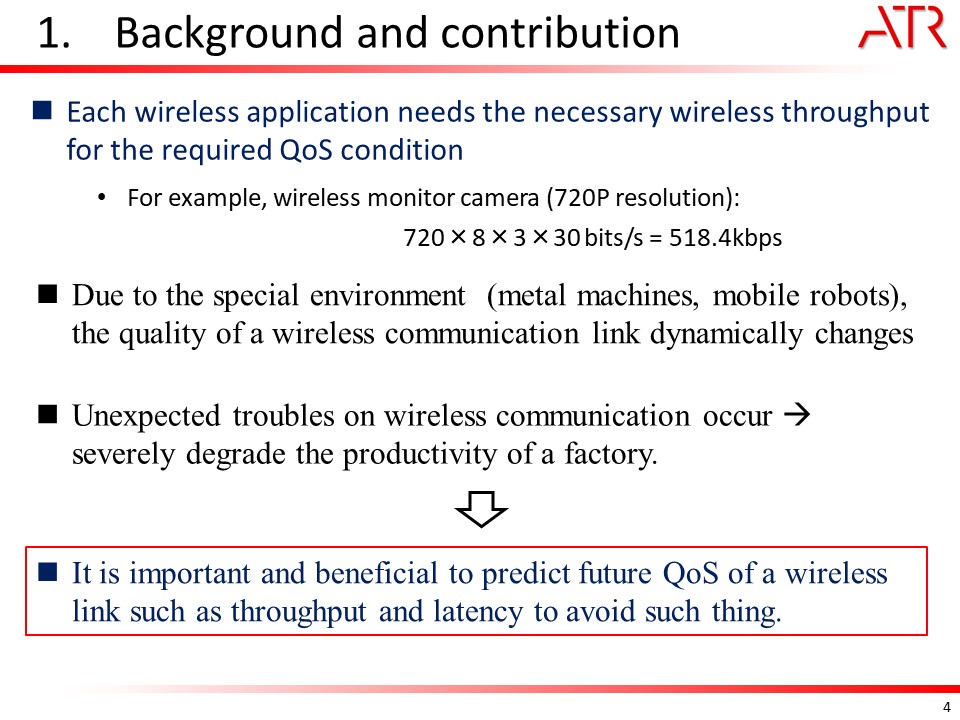 |
In addition, each wireless application needs the necessary wireless throughput for the required QoS condition. For a simple example of wireless monitor camera with 720P resolution, the required throughput can be calculated as 720×8×3×30 bits/s = 518.4kbps. That means the video data cannot be transmitted if the wireless link cannot provided such QoS condition. However, due to the special environment (metal machines, mobile robots), the quality of a wireless communication link dynamically changes. These unexpected troubles on wireless communication occur will severely degrade the productivity of a factory. Therefore, it is important and beneficial to predict future QoS of a wireless link such as throughput and latency to avoid such thing
|
|
ICACT20210223 Slide.03
[Big slide for presentation]
|
Chrome Text-to-Speach Click!! |
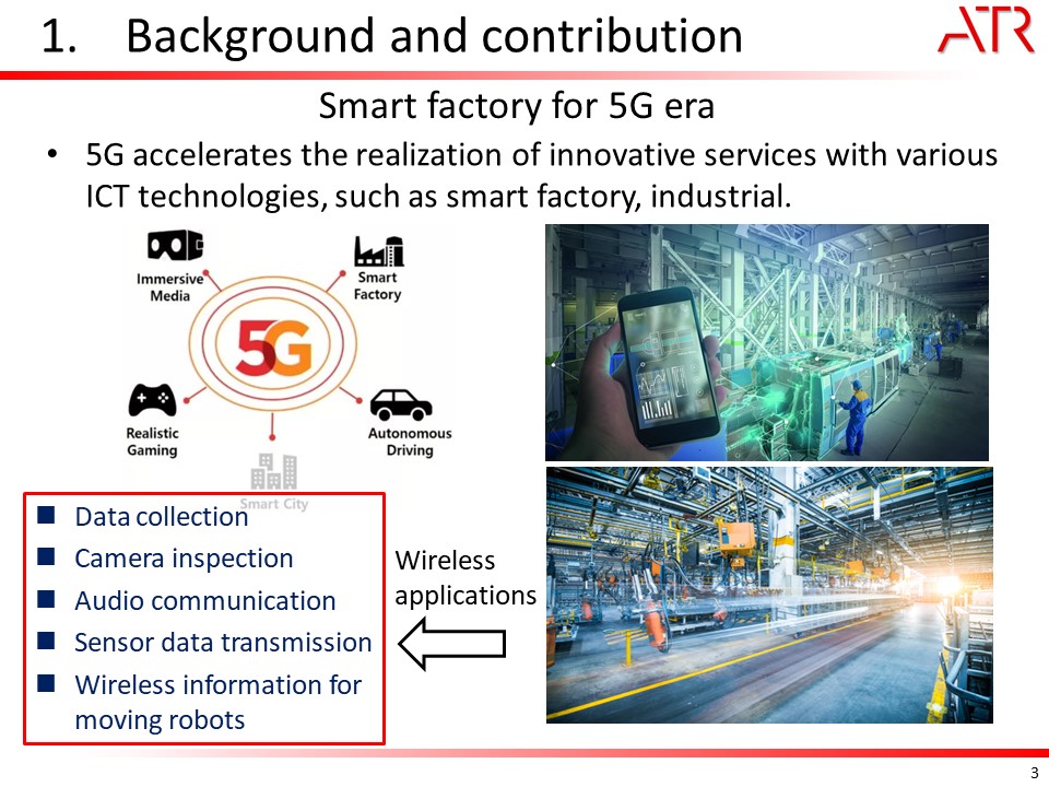 |
As we know, the era of 5G, Internet of things (IoT) and machine learning are coming which will be a boom for increasing smart usage in manufacturing sites such as factories and warehouses. In addition, 5G accelerates the realization of innovative services with various ICT technologies, such as smart factory, industrial. Therefore, it is surely that smart factory will realize many new functions with ICT technologies such as data collection, camera inspection, audio communication, sensor data transmission and wireless information for moving robots.
|
|
ICACT20210223 Slide.02
[Big slide for presentation]
|
Chrome Text-to-Speach Click!! |
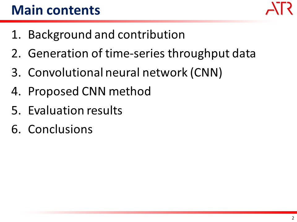 |
This presentation includes following sections. Firstly, I will explain the background and contributions of this research. Then, the generation of time-series throughput data and convolutional neural network (CNN) will be simply introduced. After that, I will talk about the major idea of our proposed CNN method. Finally, the evaluation results and conclusions will be given.
|
|
ICACT20210223 Slide.01
[Big slide for presentation]
|
Chrome Text-to-Speach Click!! |
 |
Good morning/afternoon, everyone. My name is Yafei Hou from ATR Wave Engineering Laboratory, Japan. Today, I would like to introduce our research results with the title as A Study of Throughput Prediction using Convolutional Neural Network over Factory Environment.
|