ICACT20220087 Slide.24
[Big slide for presentation] |
Chrome Text-to-Speach Click!! |
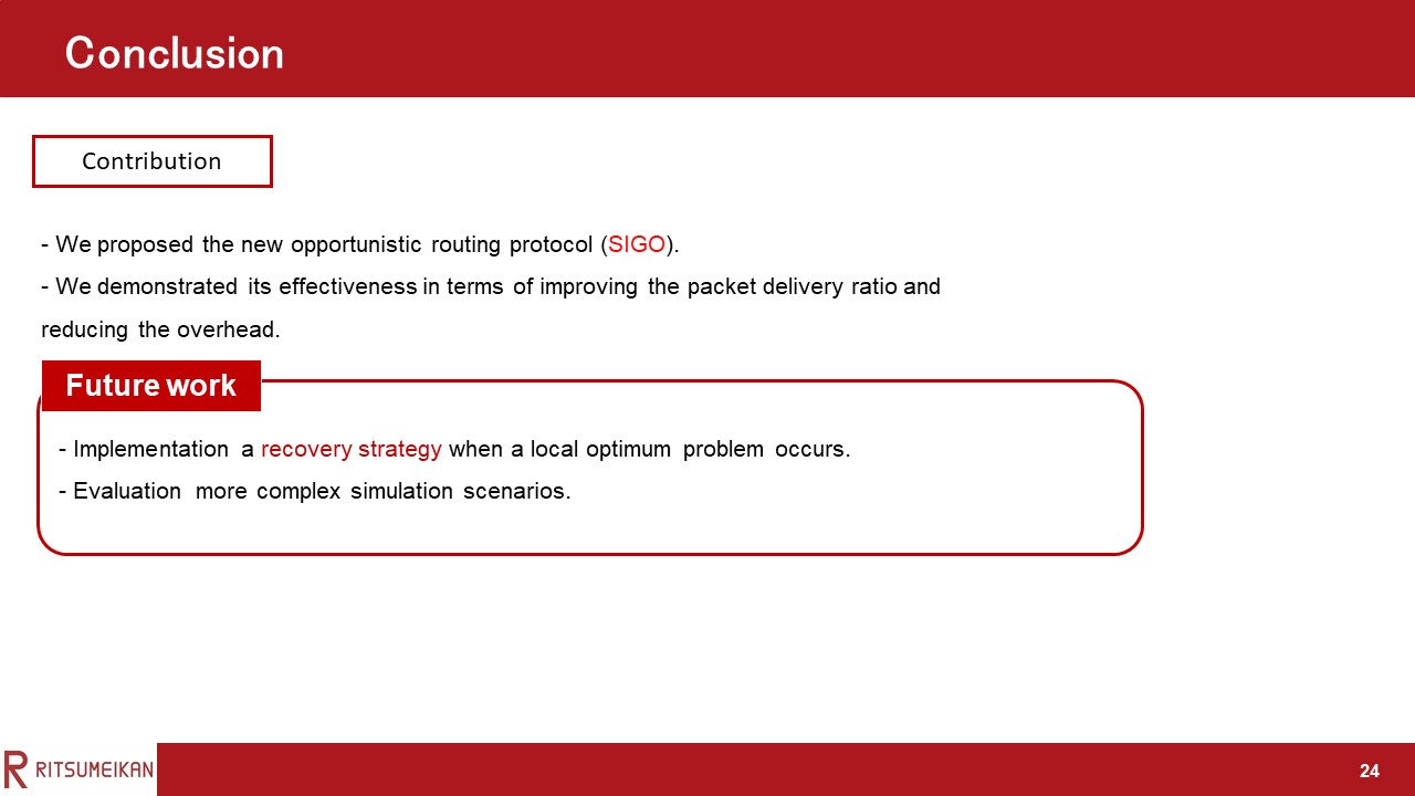 |
We proposed SIGO, which forms routes that are less susceptible to shadowing, and demonstrated its effectiveness in terms of improving the packet delivery ratio and reducing the overhead.
Future work should implement a recovery strategy when local optimum problem occurs and evaluate more complex simulation scenarios.
Thank you for listening!
|
|
ICACT20220087 Slide.23
[Big slide for presentation]
|
Chrome Text-to-Speach Click!! |
 |
Next, we describe the cause of the result.
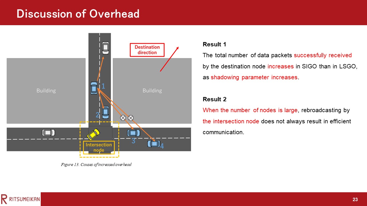
Result 1 is because that The total number of data packets successfully received by the destination node increases in SIGO than in LSGO, as shadowing parameter increases.
Result 2 is because that when the number of nodes is large, rebroadcasting by the intersection node does not always result in efficient communication.
An example is shown in this figure.
In that case, nodes on two different roads forming the intersection are likely to be selected as relay candidate nodes when the number of nodes is large. In this situation, the possibility that a low-priority candidate node cannot receive packets from a high-priority relay candidate node due to the shadowing effect of a building increases. As a result, redundant rebroadcasting increases because the rebroadcasting by a low-priority relay candidate node is not canceled. The packets rebroadcasted by the street intersection node are received by nodes 1-4. Nodes 1, 2, 3, and 4 have a higher priority in that order. Ideally, only node 1 should rebroadcast the data packet. However, even if node 1 rebroadcasts the packet, nodes 3 and 4 cannot receive it due to the shadowing effect and rebroadcast. In that case, nodes on two different roads forming the intersection are likely to be selected as relay candidate nodes when the number of nodes large.
|
|
ICACT20220087 Slide.22
[Big slide for presentation]
|
Chrome Text-to-Speach Click!! |
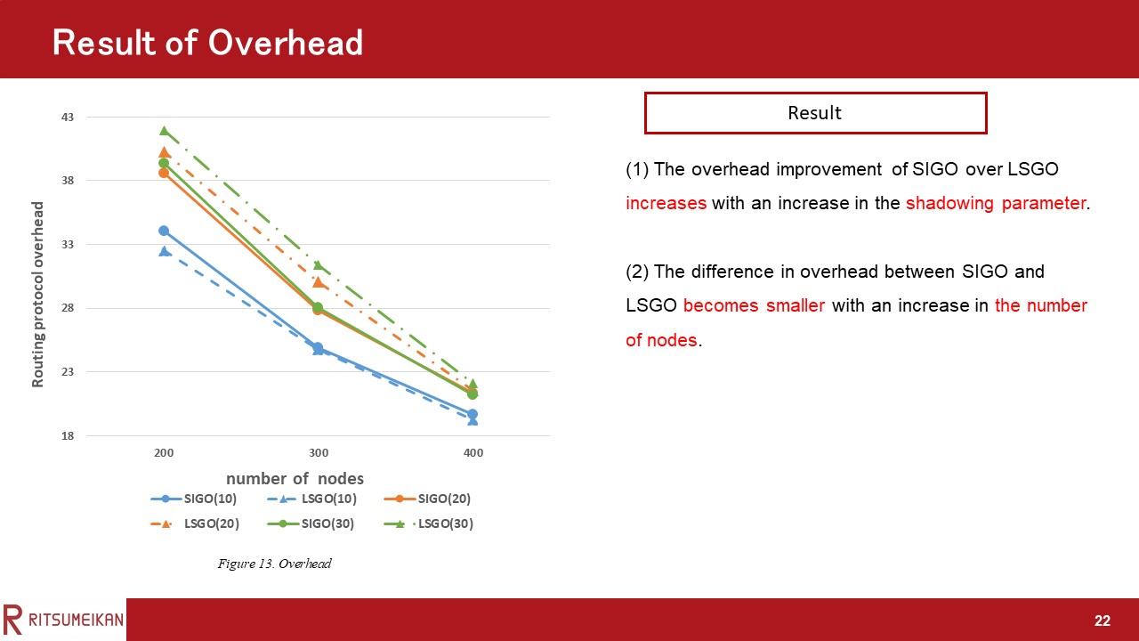 |
This figure shows the overhead.
In this evaluation, the two results were obtained.
The first is The overhead improvement of SIGO over LSGO increases with an increase in the shadowing parameter.
The second is The difference in overhead between SIGO and LSGO becomes smaller with an increase in the number of nodes.
|
|
ICACT20220087 Slide.21
[Big slide for presentation]
|
Chrome Text-to-Speach Click!! |
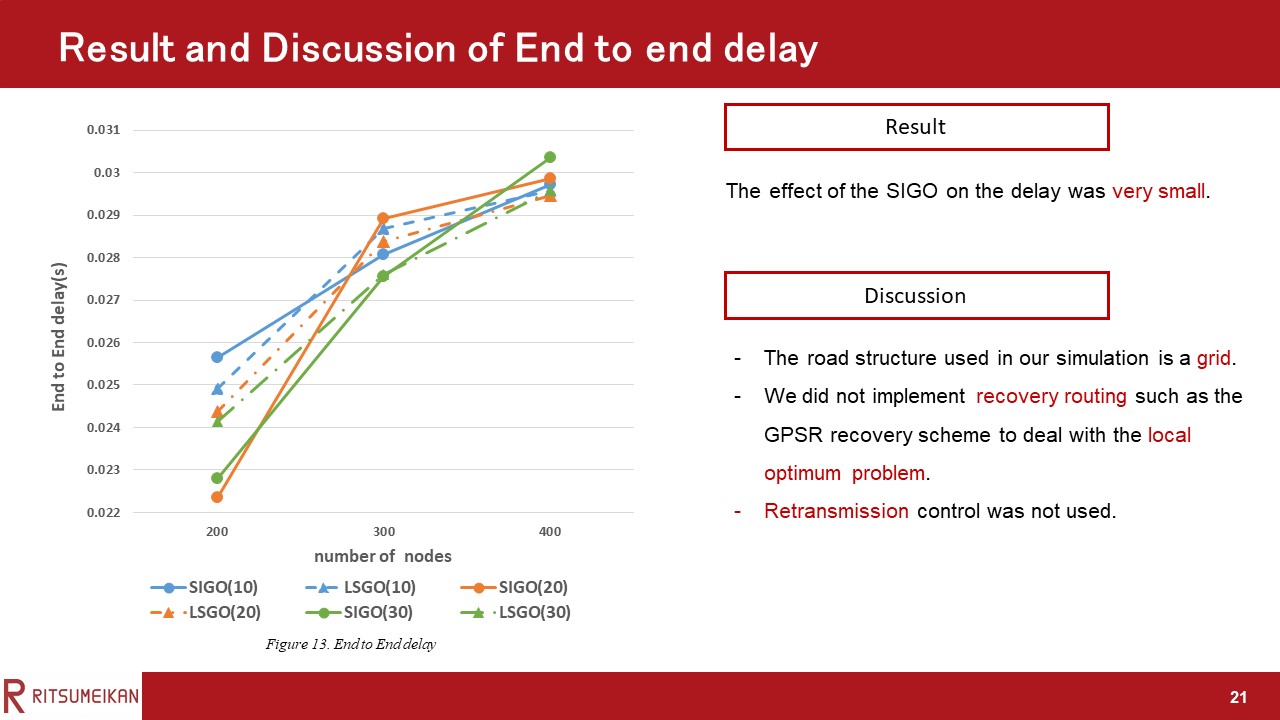 |
This Figure shows the End to end delay.
In the simulation scenario and setting of this study, the effect of the proposed protocol on the delay was very small.
We have the following three reasons for this: (1) Because the road structure used in our simulation is a grid, the distance between the source node and the destination node does not change regardless of which road the packet is relayed on. (2) In this experiment, we did not implement recovery routing such as the GPSR recovery scheme to deal with the local optimum problem. (3) Retransmission control was not used in the experiment.
|
|
ICACT20220087 Slide.20
[Big slide for presentation]
|
Chrome Text-to-Speach Click!! |
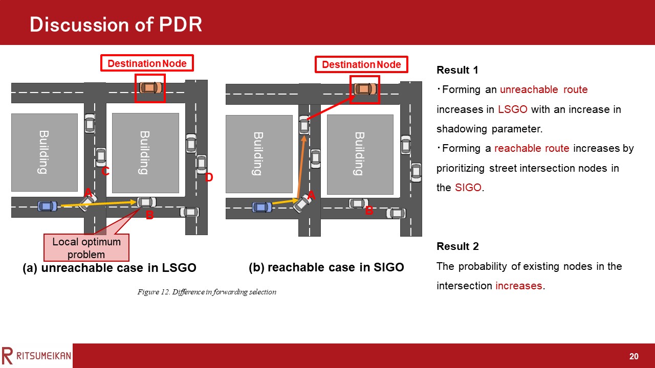 |
Next, we describe the cause of the result.
Result 1 is because the possibility of forming an unreachable route as shown in Figure (b) increases in LSGO with an increase in α. The possibility of forming a reachable route increases by prioritizing street intersection nodes in the SIGO.
Result 2 is because increasing in the probability of the existence of nodes in the intersection.
|
|
ICACT20220087 Slide.19
[Big slide for presentation]
|
Chrome Text-to-Speach Click!! |
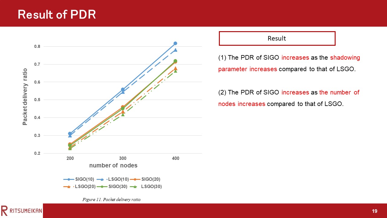 |
This Figure shows the PDR of SIGO and LSGO when the number of nodes and the shadowing parameter are varied.
The solid line shows the proposed method SIGO, and the dotted line shows the comparison method LSGO.
Also, SIGO (1) shows the PDR of the proposed protocol when the shadowing parameter is 10db.
In this evaluation, the two results were obtained.
The first is that the PDR of SIGO increases as the shadowing parameter increases compared to that of LSGO.
The second is that the PDR of SIGO increases as the number of nodes increases compared to that of LSGO.
|
|
ICACT20220087 Slide.18
[Big slide for presentation]
|
Chrome Text-to-Speach Click!! |
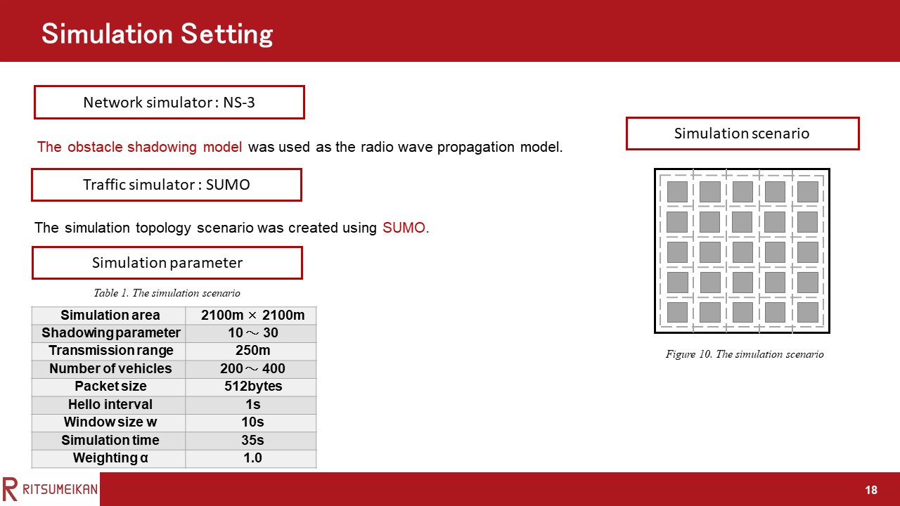 |
Next, we describe the simulation setting.
The simulation parameters are shown in Table I.
The simulation topology scenario was created using SUMO , as shown in this Figure .
Traffic signals were placed at each intersection, and buildings were placed as shown in the gray area of this Figure.
The obstacle shadowing model was used as the radio wave propagation model.
|
|
ICACT20220087 Slide.17
[Big slide for presentation]
|
Chrome Text-to-Speach Click!! |
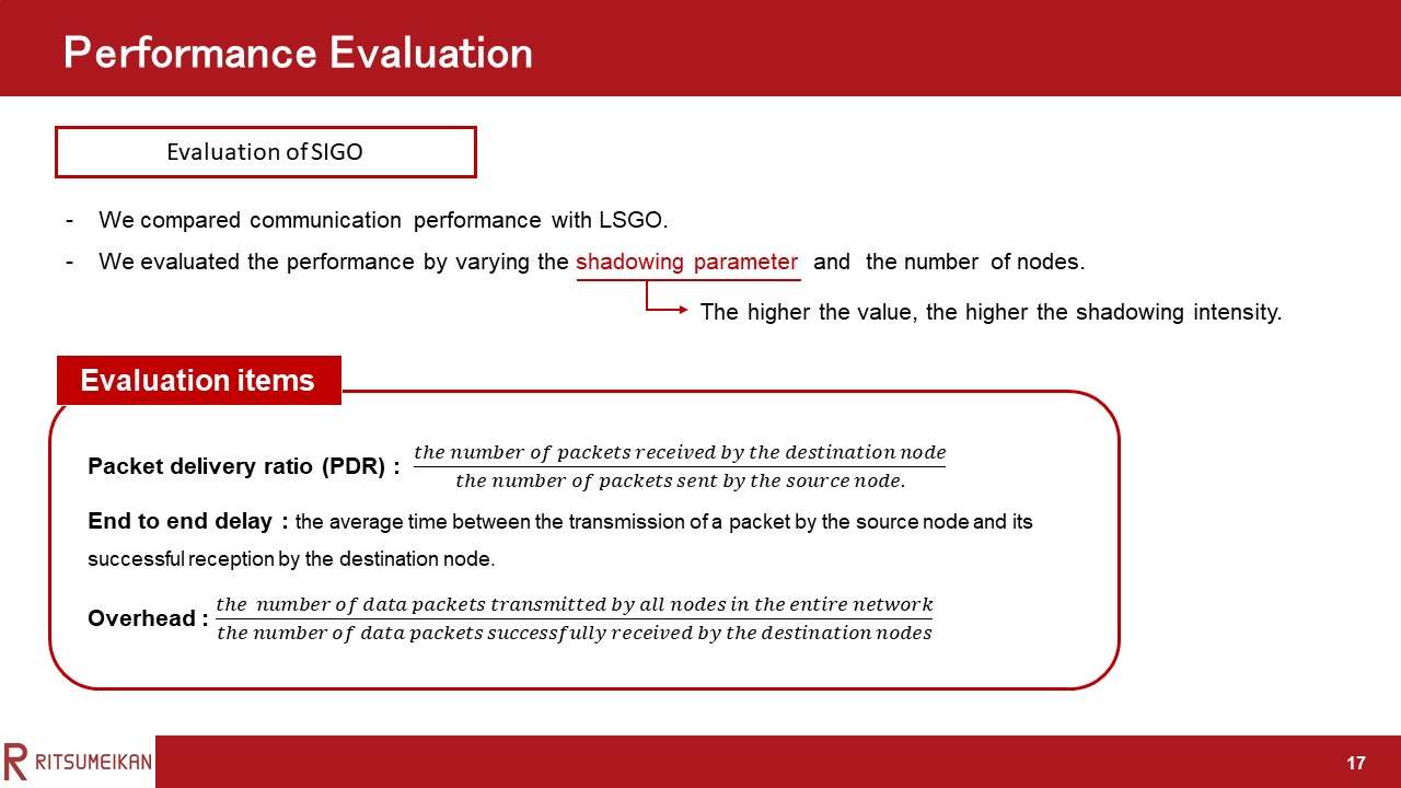 |
Here, we have the performance evaluation.
To evaluate the usefulness of the proposed protocol, we compared it with the LSGO protocol for three evaluation items: packet delivery ratio (PDR), end-to-end delay, and overhead.
We evaluated the performance by varying the shadowing parameter and the number of nodes.
The higher the shadowing parameter, the higher the shadowing intensity.
|
|
ICACT20220087 Slide.16
[Big slide for presentation]
|
Chrome Text-to-Speach Click!! |
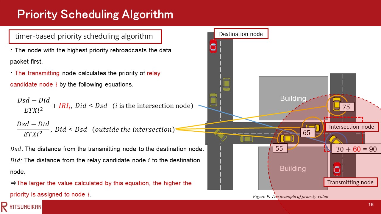 |
An example is shown in this figure. By adding the IRI, the intersection node has the highest priority in figure.
|
|
ICACT20220087 Slide.15
[Big slide for presentation]
|
Chrome Text-to-Speach Click!! |
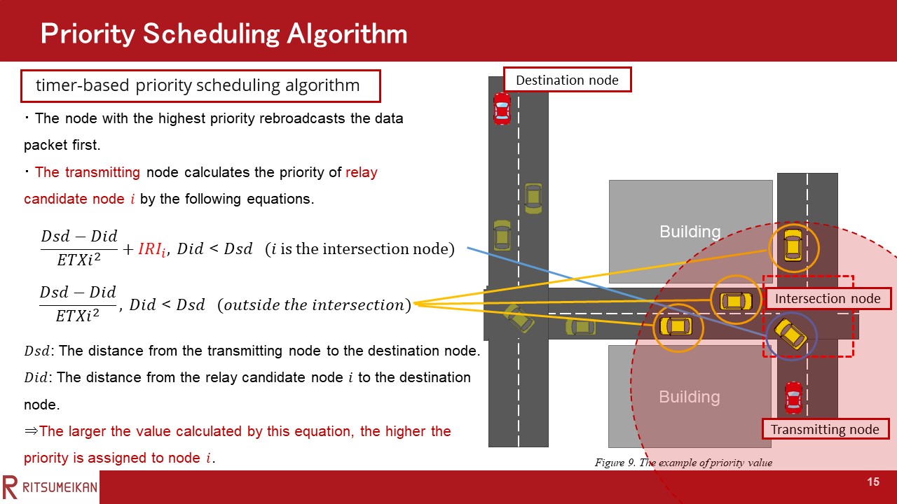 |
Next, I’d like to explain the priority scheduling algorithm.
In SIGO, a timer-based priority scheduling algorithm is used. In this algorithm, the node with the highest priority rebroadcasts the data packet first. When other relay candidate nodes overhear packets from nodes with a higher priority, they discard their pending packets. Each relay candidate node rebroadcasts the packet only when it has not received any packet from the node with a higher priority than itself until its timer expires.
The above equation is applied when node i is a street intersection node, and
the under equation is applied when node i is located outside the intersection.
The larger the value calculated by these equations, the higher the priority is assigned to node i.
|
|
ICACT20220087 Slide.14
[Big slide for presentation]
|
Chrome Text-to-Speach Click!! |
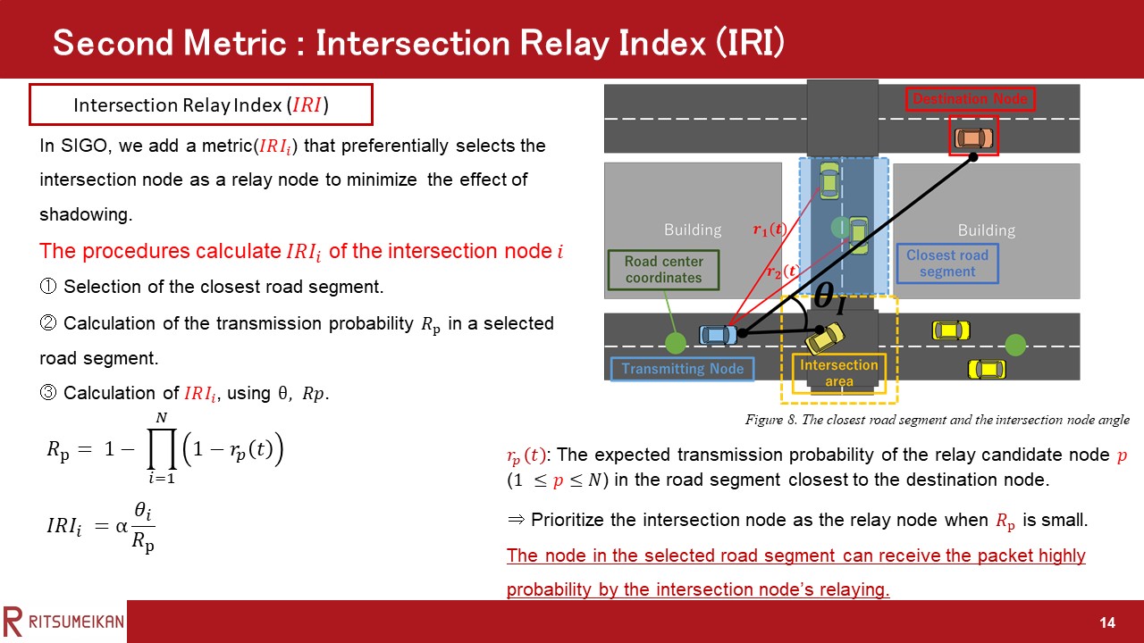 |
Next, I’d like to explain second metric in the priority determination. The second metric is the intersection relay index (IRI).
In SIGO, we add the metric that preferentially selects the intersection node as a relay node to minimize the effect of shadowing.
The following procedures calculate IRI, which gives priority to the street intersection node.
The step1 is Selection of the closest road segment.
To calculate IRI, the transmitting node (relay node or the source node) selects one of the road segments closest to the destination node among the road segments where relay candidate nodes exist.
The center coordinate of each road segment was used to calculate the distance between the destination node and road segment.
The transmitting node is relay node or the source node.
An example is shown in this Figure.
In this example, the road segment closest to the destination node is enclosed by the dashed blue line in the figure.
The step2 is Calculation of the transmission probability Rp in a selected road segment.
rp(t) is the expected transmission probability of the relay candidate node p in the road segment closest to the destination node.
N represents the number of candidate nodes in the road segment closest to the destination node.
The expected transmission probability was calculated using the same method as the previous slide.
The final step is calculation of the IRI, using θ, Rp.
The θi is the angle between the lines connecting the transmitting node to the destination node and connecting the transmitting node and the intersection node i.
The higher θi and the lower Rp, the higher the IRIi as shown in this equation.
this aims that the node in the selected road segment can receive the packet highly probability by the intersection node’s relaying when Rp is small.
In addition, since the local optimum problem occurs when θ is large, there is also the aim that actively selecting of the intersection node as a relay candidate node to prevent this.
|
|
ICACT20220087 Slide.13
[Big slide for presentation]
|
Chrome Text-to-Speach Click!! |
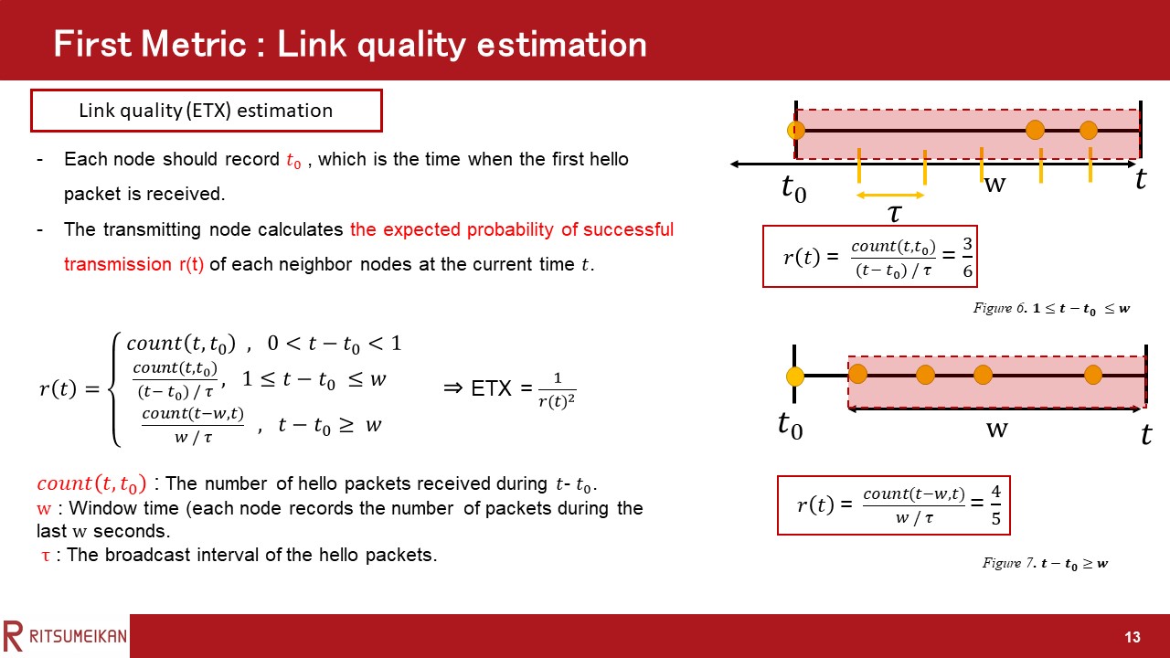 |
Next, I’d like to explain the first metric in priority determination. The first metric is link quality. To calculate the ETX of a link, each node should record t0, which is the time when the first hello packet is received and the number of packets it receives from the neighbor during the last w seconds. Then, according to the interval between t0 and the current time t and window w, the expected probability of successful transmission r(t) is calculated by the following Equation. The denominator is the number of hello packets that should have been received during the window, and τ represents the broadcast interval of the hello packets. Count (t, t0) is the number of hello packets received during t-t0. As can be seen from the equation, there are three situations in terms of the difference between t-t0 and window time w. In SIGO, the asymmetry of the link is not considered, and only the expected probability of one-way transmission is used to calculate the link ETX. Assuming that the expected probability of a one-way transmission is r(t), then the link ETX is calculated using Equation (2).
|
|
ICACT20220087 Slide.12
[Big slide for presentation]
|
Chrome Text-to-Speach Click!! |
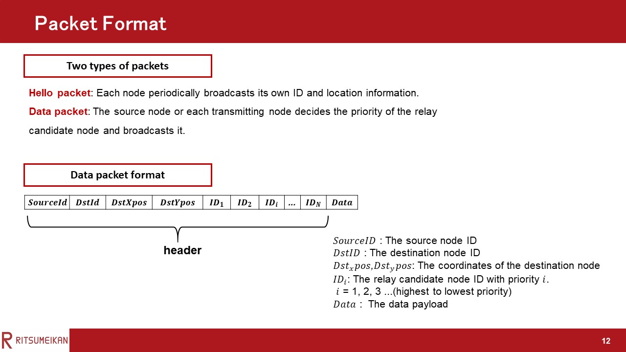 |
I’d like to start by looking at the packet format.
There are two types of packets used in SIGO.
The first is the hello packet.
In SIGO, each node periodically broadcasts a hello packet to keep track of its neighbors’ link quality and location.
The hello packet contains the ID and location information of the generating node.
The second is the data packet.
Because SIGO does not use control packets, the priority information assigned to each relay candidate node is included in the data packet. The data packet contains source node id, destination node id, destination location information, the relay candidate node ID with priority i , and data payload.
|
|
ICACT20220087 Slide.11
[Big slide for presentation]
|
Chrome Text-to-Speach Click!! |
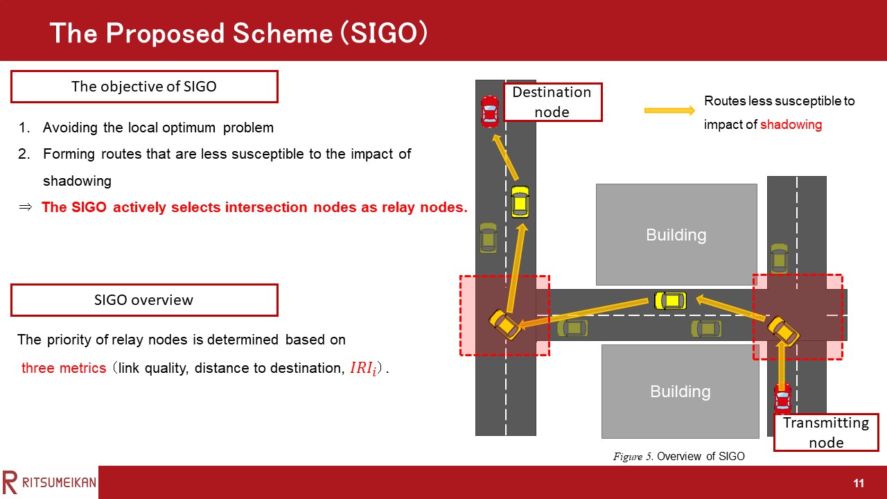 |
"Here, we have the proposed scheme.
In this study, we propose a new opportunistic routing protocol named SIGO that considers street intersections.
There are two objectives of SIGO.
The first is avoiding the local optimum problem.
The second is forming routes that are less susceptible to the impact of shadowing.
The main idea of SIGO to achieve these objectives is actively selecting intersection nodes as relay nodes.
Therefore, In SIGO, the priority of relay nodes is determined based on three metrics: distance to destination, link quality, and a street intersection relay index (IRI), which is used to give priority to nodes in the intersection.
|
|
ICACT20220087 Slide.10
[Big slide for presentation]
|
Chrome Text-to-Speach Click!! |
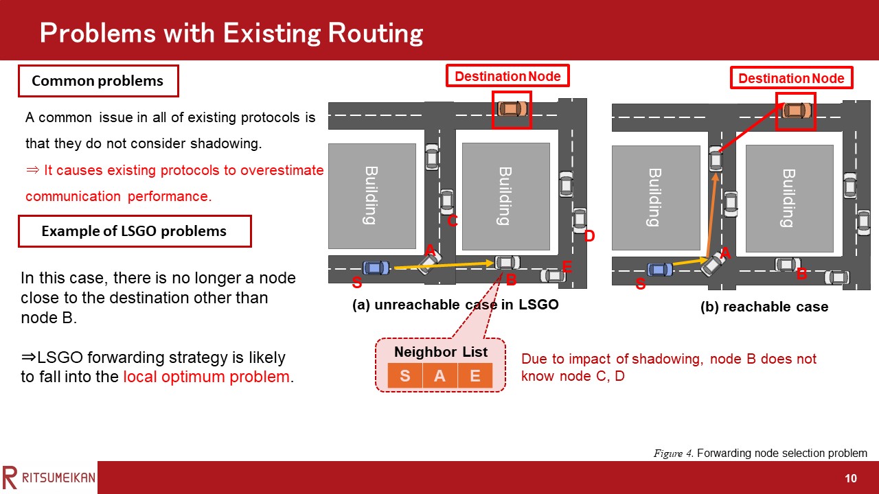 |
Here, we have problems with existing routing.
A common issue in all of existing opportunistic routing protocols is that they do not consider shadowing.
This problem causes these protocols to overestimate communication performance.
Let me use a figure to explain the example of LSGO problems.
In the forwarding strategy of LSGO, a node that is closer to the destination node and has better link quality is more likely to be selected as a forwarding node.
Consider the situation where node B is selected as the forwarding node, as shown in this Figure.
It is possible that the links with nodes C and D do not exist entirely because of shadowing in this case. In these cases, the problem is that there is no longer a node close to the destination other than node B. This has long been a problem in location-based routing protocols and is called the local optimum problem. From the above, we can see that the LSGO forwarding strategy is likely to fall into the local optimum problem and the local shadowing problem. This problem may be solved by selecting a street intersection node, such as node A, as a relay node, as shown in Figure 4 (b).
|
|
ICACT20220087 Slide.09
[Big slide for presentation]
|
Chrome Text-to-Speach Click!! |
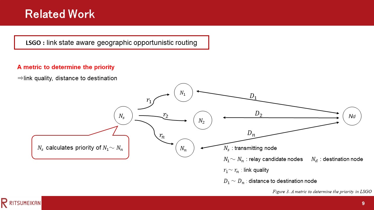 |
Here, we have related work.
LSGO has been proposed as a typical Opportunistic routing for VANETs.
In LSGO, the link quality and distance from the destination are used to determine the priority, improving communication performance.
|
|
ICACT20220087 Slide.08
[Big slide for presentation]
|
Chrome Text-to-Speach Click!! |
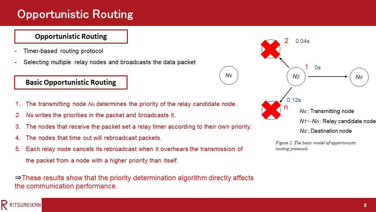 |
Step 5, Each relay node cancels its rebroadcast when it overhears the transmission of the packet from a node with a higher priority than itself before its timer expires, thereby preventing the increase of redundant packets.
These results show that in opportunistic routing protocols, the priority determination algorithm directly affects the communication performance.
|
|
ICACT20220087 Slide.07
[Big slide for presentation]
|
Chrome Text-to-Speach Click!! |
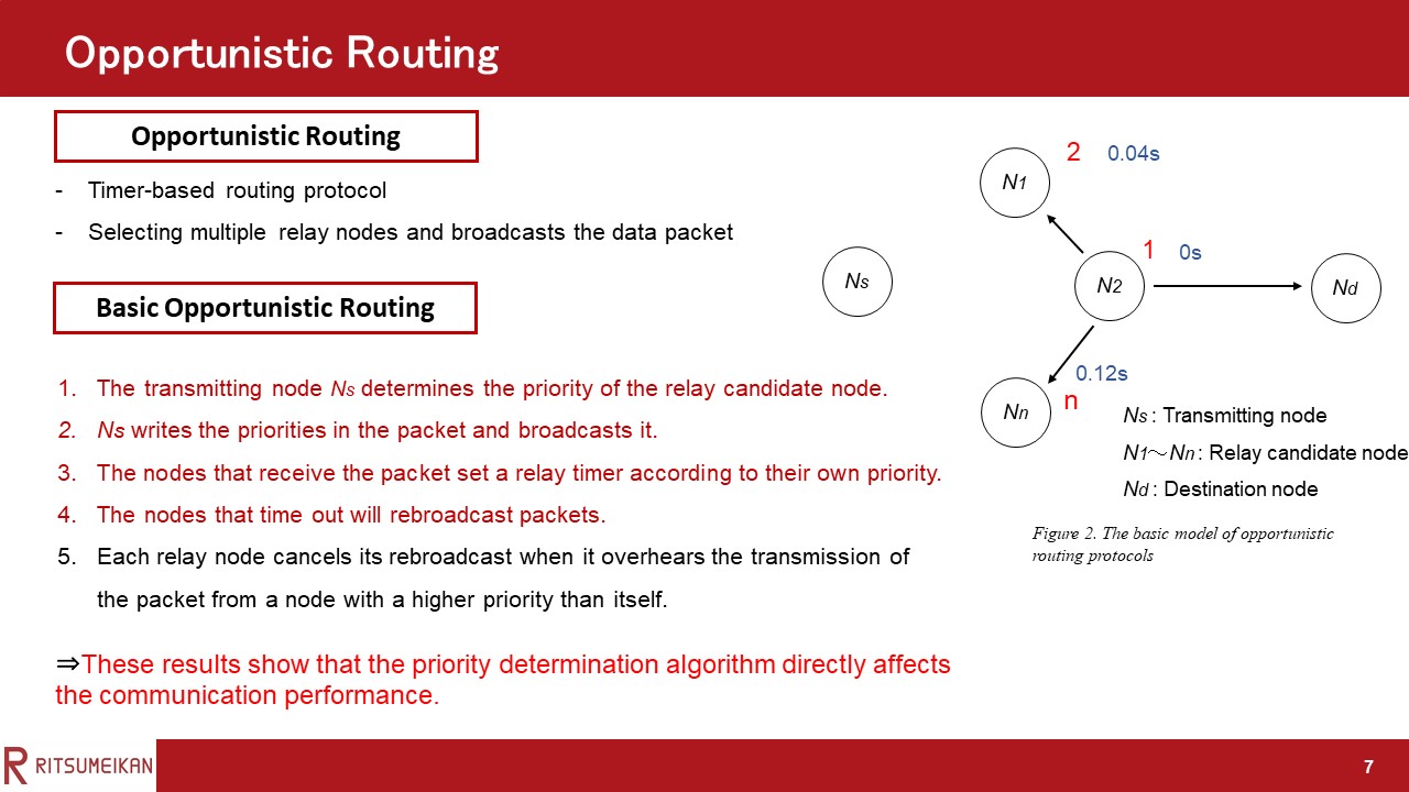 |
Step 4, The nodes that time out will rebroadcast packets.
|
|
ICACT20220087 Slide.06
[Big slide for presentation]
|
Chrome Text-to-Speach Click!! |
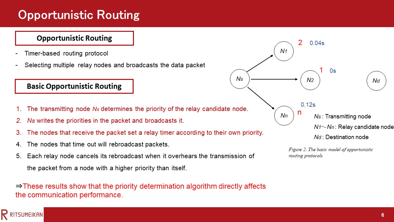 |
Step 3, The nodes that receive the packet set a relay timer according to their own priority. The higher the priority, the smaller the relay timer is set.
|
|
ICACT20220087 Slide.05
[Big slide for presentation]
|
Chrome Text-to-Speach Click!! |
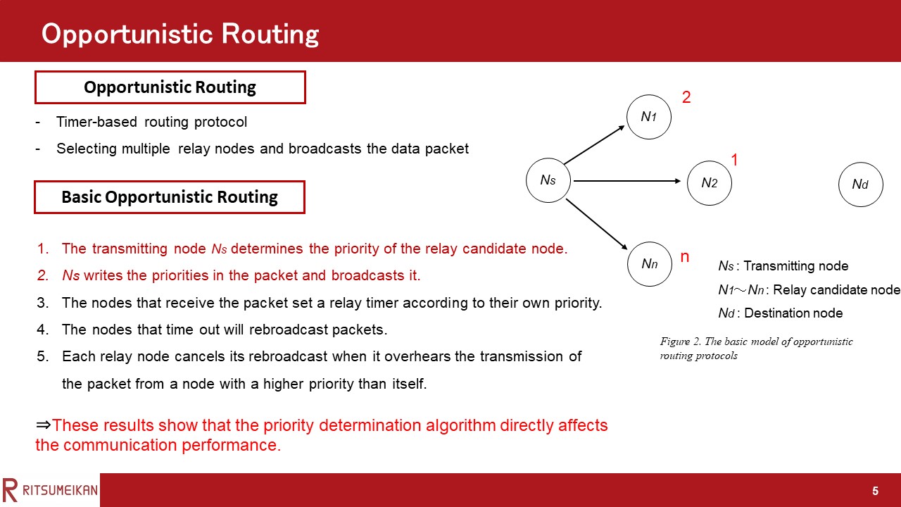 |
Step 2, Ns writes the priorities in the packet and broadcasts it.
|
|
ICACT20220087 Slide.04
[Big slide for presentation]
|
Chrome Text-to-Speach Click!! |
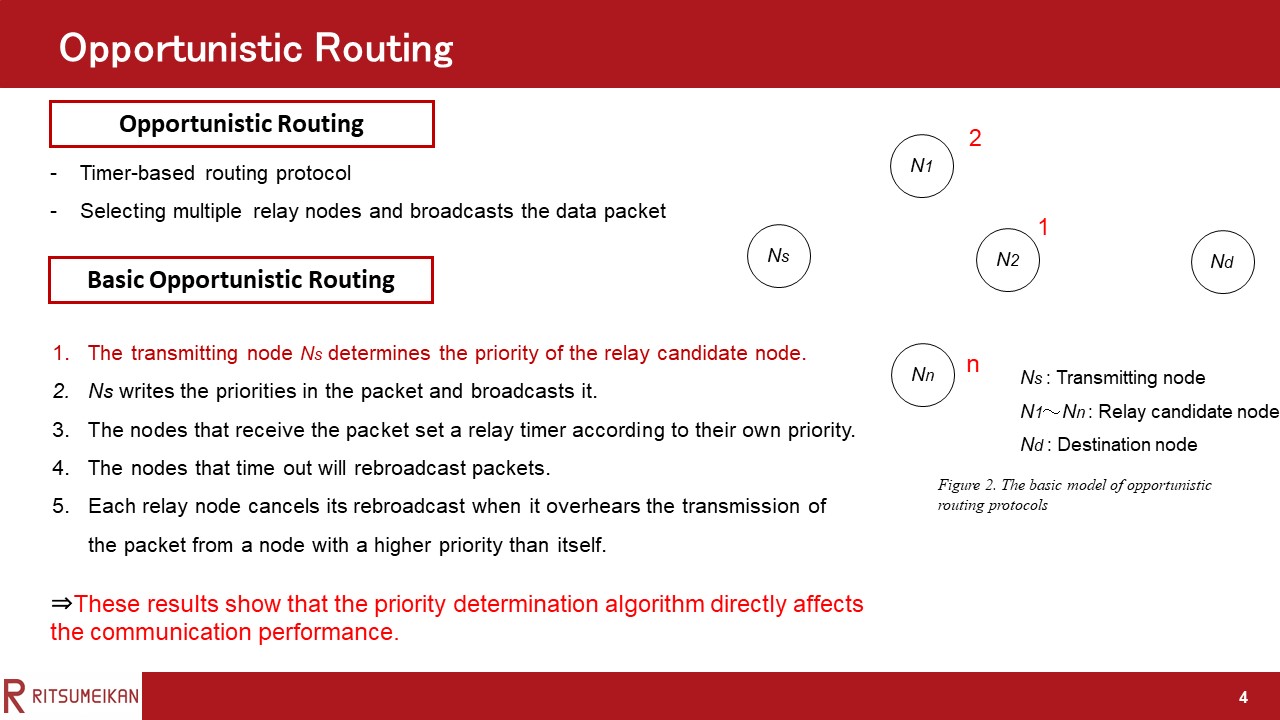 |
Step 1, The transmitting node Ns selects a candidate node for relaying and determines the priority from N1 to Nn.
|
|
ICACT20220087 Slide.03
[Big slide for presentation]
|
Chrome Text-to-Speach Click!! |
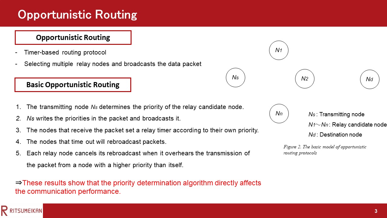 |
This section describes the basic opportunistic routing flow.
The routing protocol for VANETs has to meet various requirements.
Therefore, In recent years, Opportunistic routing protocol has been attracting attention.
The opportunistic routing protocol broadcasts the data packet using multiple relay nodes, as opposed to the traditional geographic routing protocol.
This section describes the basic opportunistic routing flow.
|
|
ICACT20220087 Slide.02
[Big slide for presentation]
|
Chrome Text-to-Speach Click!! |
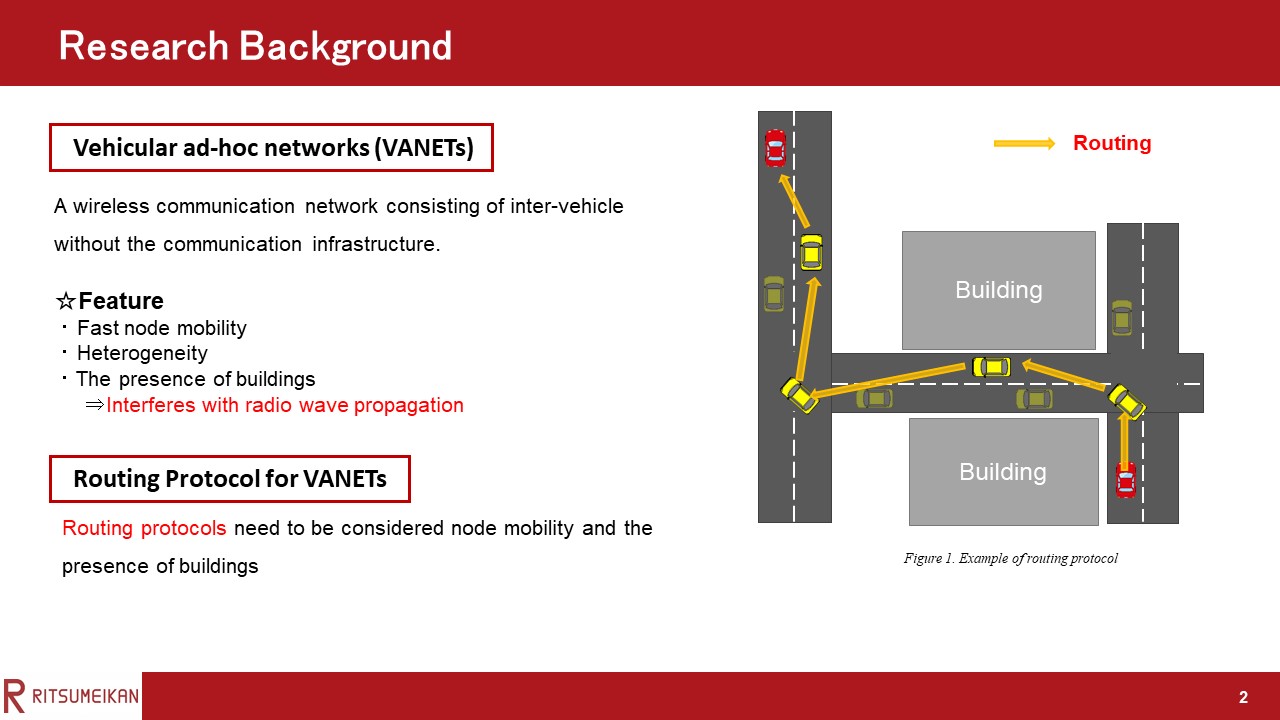 |
Here, we have resarch backgrounds. VANETs is ad-hoc-communication between vehicles equipped with wireless communication devices. It enables the construction of flexible networks. As shown in Figure 1, VANETs allow data to be delivered to distant vehicles using vehicle-to-vehicle routing, without the communications infrastructure. When VANETs are deployed in urban environments, fast node mobility, heterogeneity, and the presence of buildings must be considered in the performance evaluation.
|
|
ICACT20220087 Slide.01
[Big slide for presentation]
|
Chrome Text-to-Speach Click!! |
 |
Hi everybody, my name is Shuto Takahashi. I'm from ritumeikan university in japan.
It is a great honor to be able to speak to you today.
Today I’d like to talk about routing protocol that minimizes the effect of shadowing for VANETs.
|