ICACT20240426 Slide.22
[Big slide for presentation]
[YouTube] |
Chrome Text-to-Speach Click!! |
 |
Thanks for your attention!
|
|
ICACT20240426 Slide.21
[Big slide for presentation]
[YouTube] |
Chrome Text-to-Speach Click!! |
 |
Now! The floor is open for Questions and Answers. Welcome any comment or question.
|
|
ICACT20240426 Slide.20
[Big slide for presentation]
[YouTube] |
Chrome Text-to-Speach Click!! |
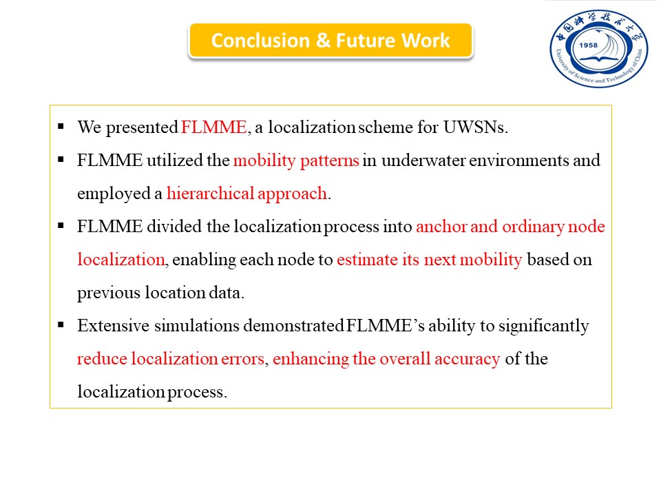 |
We presented FLMME, a localization scheme for UWSNs.
FLMME utilized the mobility patterns in underwater environments and employed a hierarchical approach.
FLMME divided the localization process into anchor and ordinary node localization, enabling each node to estimate its next mobility based on previous location data.
Extensive simulations demonstrated FLMME’s ability to significantly reduce localization errors, enhancing the overall accuracy of the localization process.
|
|
ICACT20240426 Slide.19
[Big slide for presentation]
[YouTube] |
Chrome Text-to-Speach Click!! |
 |
Finally, the Conclusions & Future Work
|
|
ICACT20240426 Slide.18
[Big slide for presentation]
[YouTube] |
Chrome Text-to-Speach Click!! |
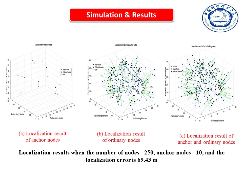 |
Fourth, the localization results when the number of nodes is 250. As we can see, Figure (a) presents the movement of the anchor nodes. While Figure (b) shows the relation between the estimated and the actual locations of the ordinary nodes with an average localization error of 69.43 m. In contrast, Figure (c) presents the localization results for all anchors and ordinary nodes. As we can see from the results that increasing the node density leads to decreasing the average localization error and, therefore, increasing the localization accuracy of our method.
|
|
ICACT20240426 Slide.17
[Big slide for presentation]
[YouTube] |
Chrome Text-to-Speach Click!! |
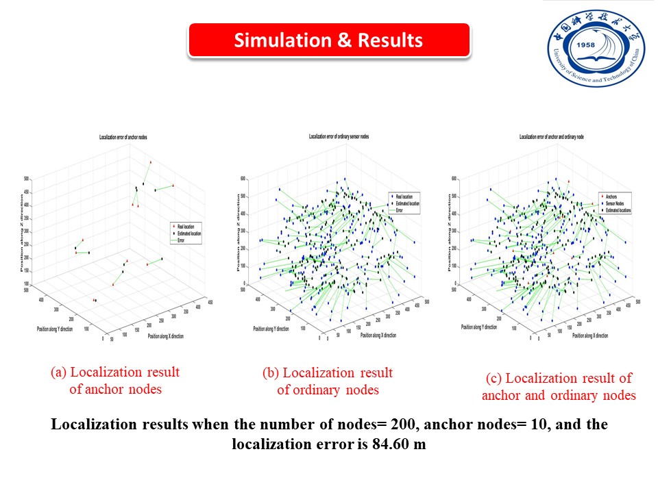 |
Third, the localization results when the number of nodes is 200. As we can see, Figure (a) presents the movement of the anchor nodes. While Figure (b) shows the relation between the estimated and the actual locations of the ordinary nodes with an average localization error of 84.60 m. In contrast, Figure (c) presents the localization results for all anchors and ordinary nodes.
|
|
ICACT20240426 Slide.16
[Big slide for presentation]
[YouTube] |
Chrome Text-to-Speach Click!! |
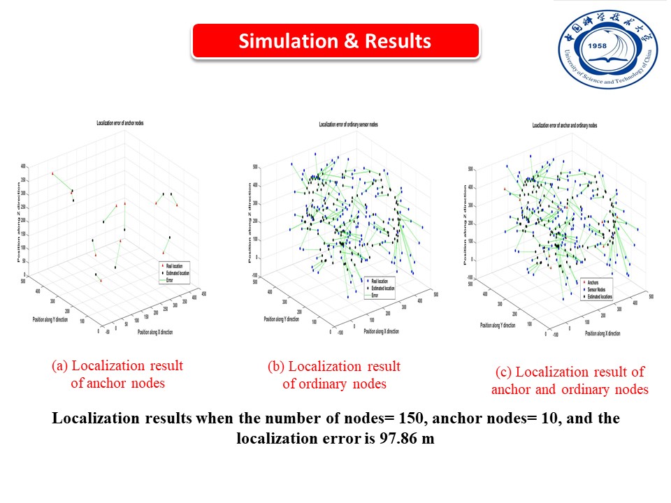 |
Second, the localization results when the number of nodes is 150. As we can see, Figure (a) presents the movement of the anchor nodes. While Figure (b) shows the relation between the estimated and the actual locations of the ordinary nodes with an average localization error of 97.86 m. In contrast, Figure (c) presents the localization results for all anchors and ordinary nodes.
|
|
ICACT20240426 Slide.15
[Big slide for presentation]
[YouTube] |
Chrome Text-to-Speach Click!! |
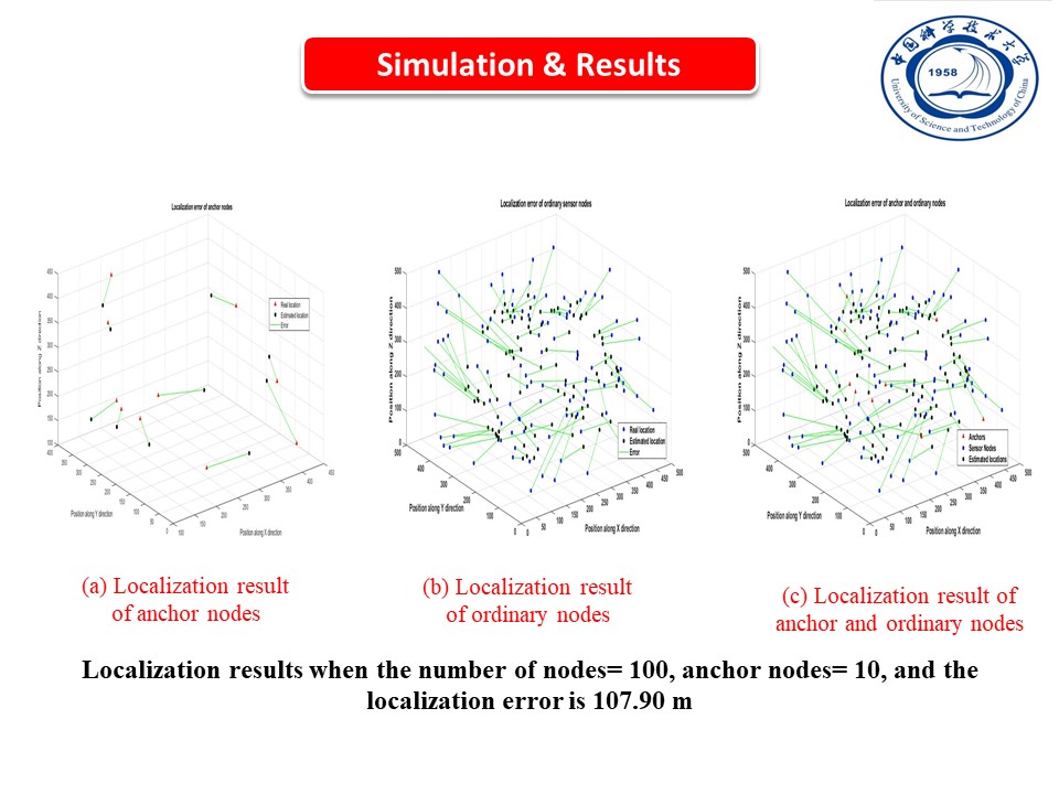 |
We analyze the impact of the node density (increasing the number of nodes from 100 to 250 ordinary nodes) on the localization performance.
First, the localization results when the number of nodes is 100. As we can see, Figure (a) presents the movement of the anchor nodes. While Figure (b) shows the relation between the estimated and the actual locations of the ordinary nodes with an average localization error of 107.90 m. In contrast, Figure (c) presents the localization results for all anchors and ordinary nodes.
|
|
ICACT20240426 Slide.14
[Big slide for presentation]
[YouTube] |
Chrome Text-to-Speach Click!! |
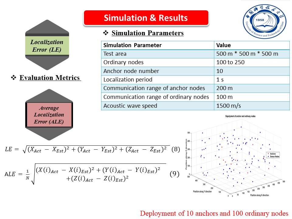 |
First, we conducted MATLAB simulations to evaluate the efficiency of FLMME. The simulation parameters are shown in this Table. We deployed 100 to 250 ordinary sensor nodes and 10 anchor nodes in a 3D area of size 500m * 500m * 500m. We set the communication range of ordinary nodes to 200m, and the acoustic wave speed to 1500 m/s. This figure shows the deployment of the anchor nodes and the ordinary nodes at the
beginning of the simulation.
Evaluation metrics: to validate the localization accuracy of the FLMME, we used two metrics: (1) the localization error (LE) given by equation (8) and the average localization error (ALE) given by equation (9).
|
|
ICACT20240426 Slide.13
[Big slide for presentation]
[YouTube] |
Chrome Text-to-Speach Click!! |
 |
Now, we will show the simulation settings and then describe the obtained results.
|
|
ICACT20240426 Slide.12
[Big slide for presentation]
[YouTube] |
Chrome Text-to-Speach Click!! |
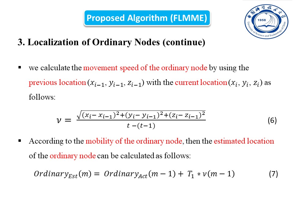 |
Continue Localization of Ordinary Nodes. After calculating the initial locations of ordinary nodes. Now, We calculate the movement speed of the ordinary node by using the previous location (𝑥_(𝑖−1), 𝑦_(𝑖−1), 𝑧_(𝑖−1)) with the current location (𝑥_𝑖, 𝑦_𝑖, 𝑧_𝑖) as given by equation (6). After that, according to the mobility of the ordinary node, then the estimated location of the ordinary node can be calculated by equation (7).
|
|
ICACT20240426 Slide.11
[Big slide for presentation]
[YouTube] |
Chrome Text-to-Speach Click!! |
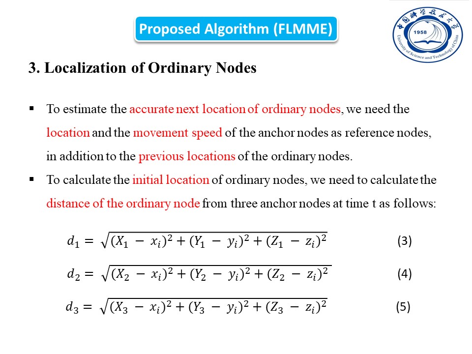 |
Localization of Ordinary Nodes. Now, we will estimate the next location of the ordinary nodes. To estimate the accurate next location of ordinary nodes, we need the location and the movement speed of the anchor nodes as reference nodes, in addition to the previous locations of the ordinary nodes. Unlike the anchor nodes that know their initial locations, the ordinary nodes do not know their initial locations. Therefore, to calculate the initial location of ordinary nodes, we need to calculate the distance of the ordinary node from three anchor nodes at time t as given by equations (3), (4), and (5).
|
|
ICACT20240426 Slide.10
[Big slide for presentation]
[YouTube] |
Chrome Text-to-Speach Click!! |
 |
Mobility Estimation of Anchor Nodes.
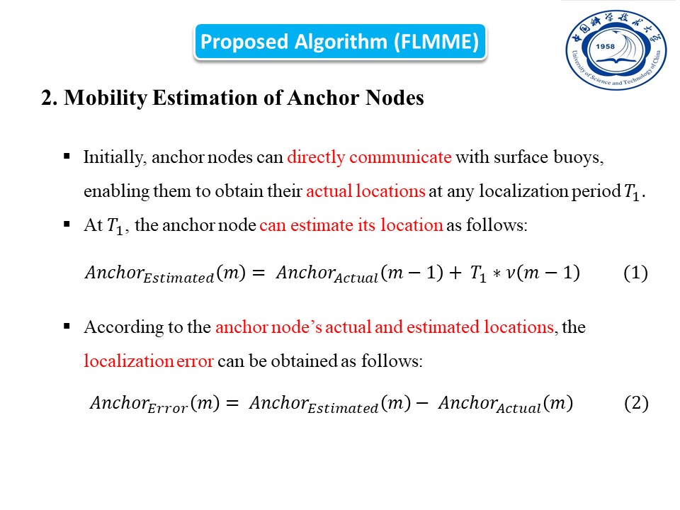
This is the first step in FLMME, in which we will estimate the mobility of the anchor nodes and then estimate the location of the anchor nodes in localization period T1. Initially, anchor nodes can directly communicate with surface buoys, enabling them to obtain their actual locations at any localization period T1. Additionally, these nodes can estimate their next mobility patterns based on previous measurements. In the localization period T1, the anchor node can estimate its location by equation (1). Then, according to the anchor node’s actual and estimated locations, the localization error can be obtained by equation (2). Then, the anchor node can assist in the localization of ordinary nodes.
|
|
ICACT20240426 Slide.09
[Big slide for presentation]
[YouTube] |
Chrome Text-to-Speach Click!! |
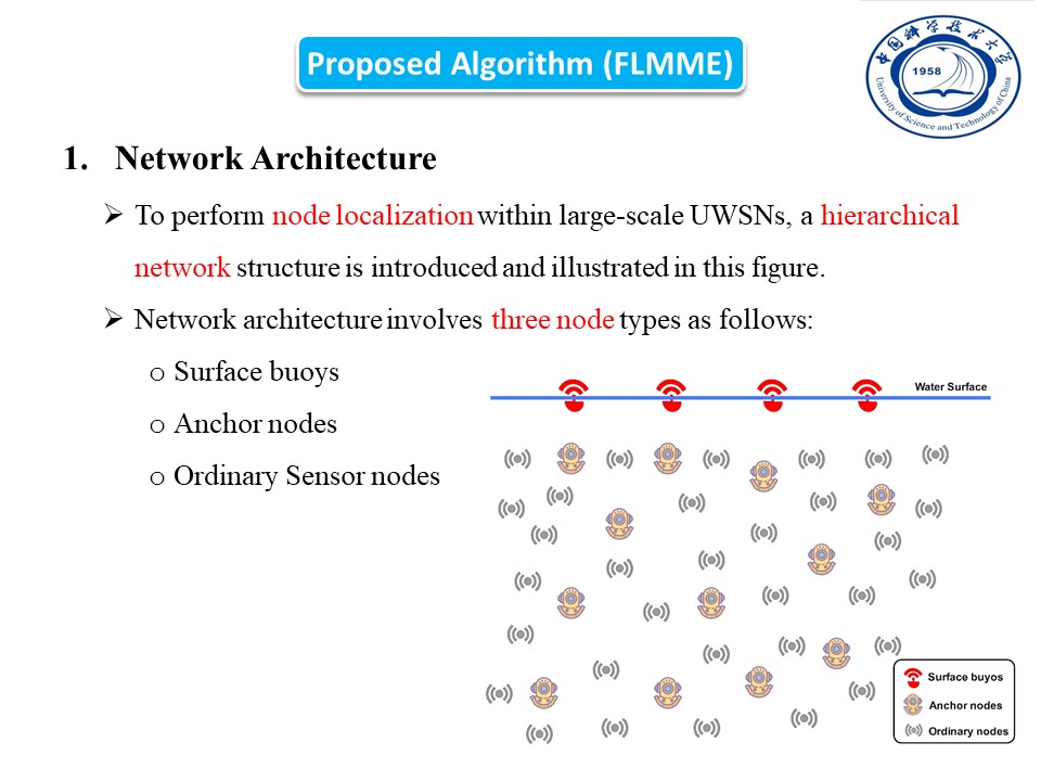 |
First, we explain the network architecture. To perform node localization within large-scale UWSNs, we introduce a hierarchical network structure, as seen in the figure. The network architecture contains three node types as follows: (1) Surface buoys that are located on the ocean surface and achieve precise location data through GPS systems. (2) Anchor nodes are high-energy devices that communicate directly with buoy nodes to determine their positions. They move in concurrence with the water current. (3) Ordinary Sensor nodes: similar to anchor nodes, these ordinary nodes inertly drift with the water current. They are unable to connect with buoys directly and are not all within the coverage of anchor nodes.
|
|
ICACT20240426 Slide.08
[Big slide for presentation]
[YouTube] |
Chrome Text-to-Speach Click!! |
 |
Next, I will explain the Proposed Algorithm (FLMME). FLMME utilizes a hierarchical localization strategy. FLMME separates the overall localization procedure into two parts: (1) localization of anchor node and (2) localization of ordinary node. I will explain each part in detail in the following slides.
|
|
ICACT20240426 Slide.07
[Big slide for presentation]
[YouTube] |
Chrome Text-to-Speach Click!! |
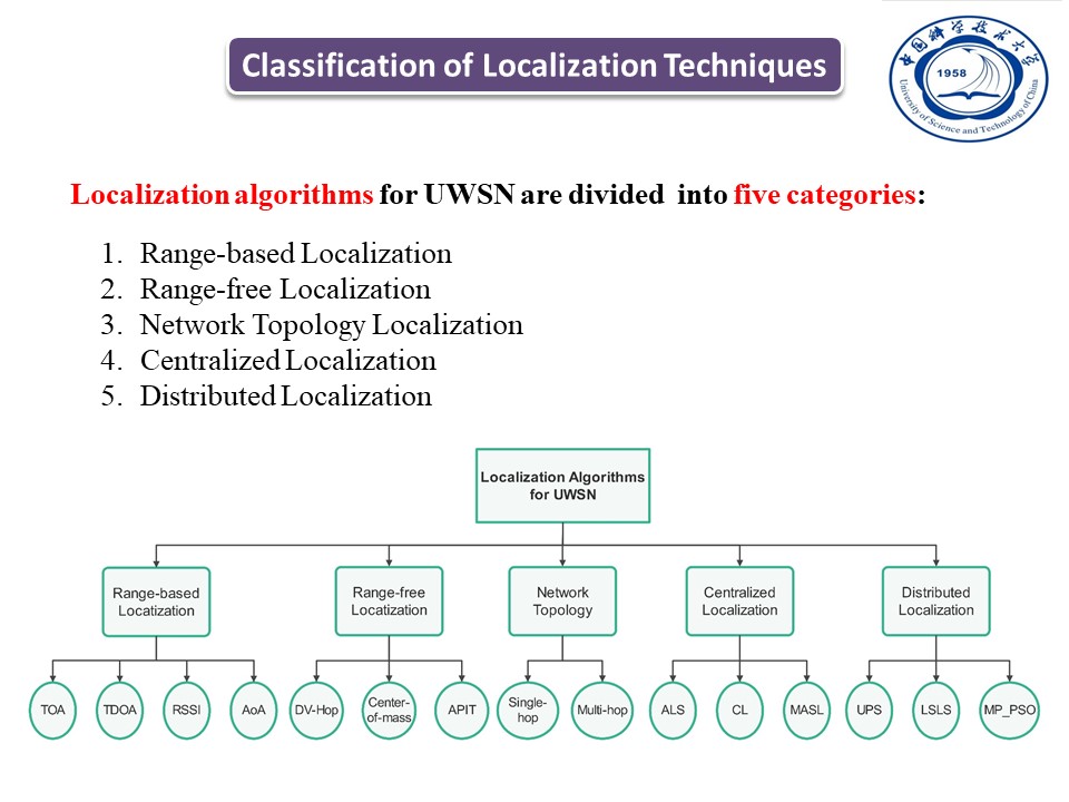 |
We divided the localization algorithms for UWSNs into five categories:(1) range-based, (2) range-free, (3) network-based topology, (4) centralized, and (5) distributed localization schemes, as seen in this figure. Here is an explanation for each category:
(1) The ranging-based algorithm employs varied techniques, such as Angle of Arrival (AOA), Time of Arrival (TOA), Received Signal Strength Indication (RSSI), and Time Difference of Arrival (TDOA), to measure node distances to anchor nodes and determine unknown node locations. (2) The range-free algorithms estimate node distances based on hop count and directional data, converting this information into approximate node positions. (3) The network-based topology localization, in which the localization algorithms are categorized into two primary types based on network topology and node connectivity: single-hop and multi-hop. (4) In a centralized localization approach, all nodes transmit collected data to a central
sink node for processing. (5) The distributed localization
method involves nodes processing their information autonomously and then interchanging this data for localization, making it ideal for large-scale UWSNs. This enables real-time node position retrieval while distributing computational tasks across the network.
|
|
ICACT20240426 Slide.06
[Big slide for presentation]
[YouTube] |
Chrome Text-to-Speach Click!! |
 |
Classification of Localization Techniques
|
|
ICACT20240426 Slide.05
[Big slide for presentation]
[YouTube] |
Chrome Text-to-Speach Click!! |
 |
Our contributions: First, we introduce an approach for underwater sensor network localization, which we call a Flexible Localization Method with Motion Estimation (FLMME). Second, FLMME employs a hierarchical localization process by dividing it into two stages: localization of anchor nodes and localization of ordinary sensor nodes. Third, each node in the localization process makes predictions about its next movement patterns based on prior known location data, enabling it to estimate its next location.
|
|
ICACT20240426 Slide.04
[Big slide for presentation]
[YouTube] |
Chrome Text-to-Speach Click!! |
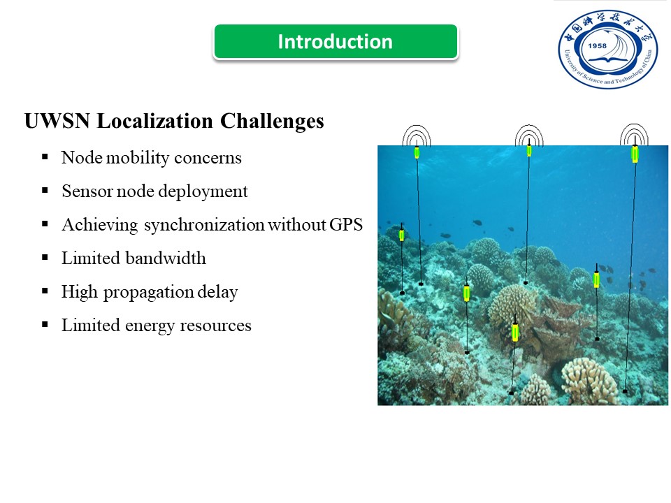 |
There are major challenges for underwater localizations, including (1) node mobility concerns driven by water currents, turbulence, and winds that displace sensor nodes from their positions. (2) Sensor node deployment is critical in network establishment but challenging in harsh underwater conditions. (3) Achieving synchronization without GPS signals poses a challenge, leading to significant localization errors in time-of-arrival-based ranging due to lack of synchronization. (4) Limited bandwidth since RF signals can not be used for communication in UWSN, but use acoustic signals for communication which has very limited bandwidth. (5) High propagation delay, since the propagation speed of the acoustic signals is less than the RF signals, resulting in significant propagation delays. (6) Limited energy since sensor nodes are equipped with small batteries that are very difficult to recharge or replace.
|
|
ICACT20240426 Slide.03
[Big slide for presentation]
[YouTube] |
Chrome Text-to-Speach Click!! |
 |
Why Underwater wireless sensor networks (UWSNs)?
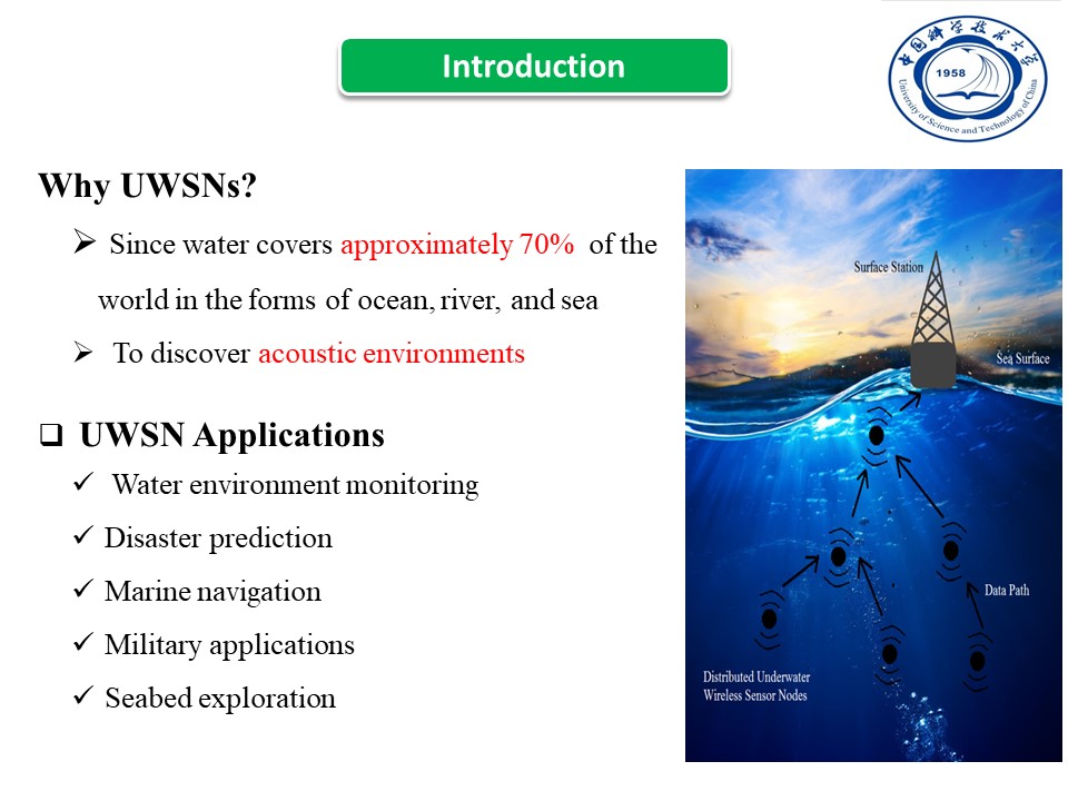
Recently, underwater wireless sensor networks become an interesting research area because water covers approximately 70% of the world in a variety of forms like ocean, river, and sea. Therefore, UWSNs are used to discover acoustic environments.
UWSNs Applications:
UWSNs are widely applied in (1) Water environment monitoring, (2) Disaster prediction, (3) Marine navigation, (4) Military applications, and (5) Seabed exploration.
|
|
ICACT20240426 Slide.02
[Big slide for presentation]
[YouTube] |
Chrome Text-to-Speach Click!! |
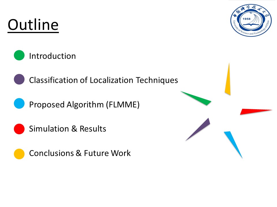 |
The outline of our presentation is as follows: first, give a brief introduction about the importance of UWSNs and their applications. Second, describe the classification of localization techniques for UWSNs. Third, describe our proposed method, which is FLMME. Fourth, the simulation and results. Finally, the conclusion of our paper and the future work.
|
|
ICACT20240426 Slide.01
[Big slide for presentation]
[YouTube] |
Chrome Text-to-Speach Click!! |
 |
Hello everyone; my name is Abdelrahman Samy. Today, I'm going to present our paper under the title " Flexible Localization Method with Motion Estimation for Underwater Wireless Sensor Networks."
|