Now 4260 visitors
Today:0 Yesterday:0
Total: 142772
215S 51P 5R
2026-10-21, Week 43 |
| Member Login |
| TACT Journal Homepage |
| Call for Paper |
| Committee |
| Find My Paper |
| Author Homepage |
| Statistics & History |
| Welcome Message |
| Paper Procedure |
| FAQ |
| Paper Archives |
| Outstanding Papers |
| Author Homepage |
| - Paper Procedure |
| - Journal Procedure |
| - Presentation Tips |
|
| Program & Proceedings |
| Program with Papers |
| Plenary Session |
| Tutorial Session |
|
| Presentation Platform |
| Hotel & Travel Info |
| About Korea |
| Accommodation |
| Transportation |
| VISA |
| Other Infomation |
|
| Photo Gallery |
| Scheduler Login |
| Seminar |
| Archives Login |
|
| Sponsors |

|

|

|

|

|
|

|

|
|

|
|
|
|
|
 ICACT20210129 Slide.01
[Big Slide] |
Chrome  Click!! |
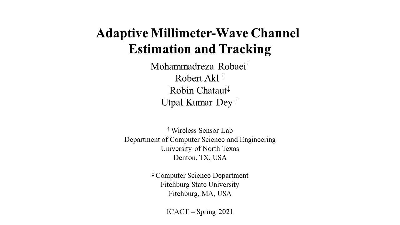 |
Good morning. Thanks for coming to this presentation. My name is Mohammdareza Robaei. I am Ph.D. candidate at the Computer Science and Engineering Department, University of North Texas, USA. Our presentation is about adaptive millimeter-wave channel estimation and tracking.
|
| ICACT20210129 Slide.02
[Big Slide]
|
Chrome Click!! |
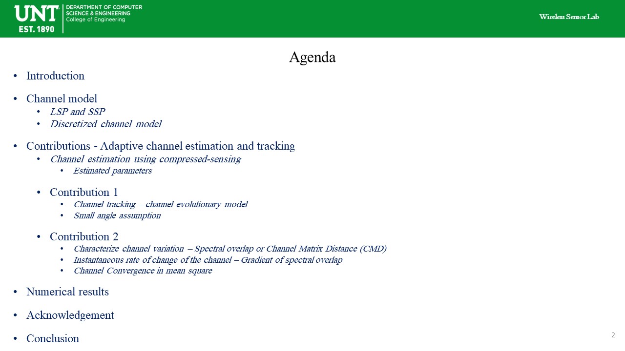 |
Our agenda is as in the following. We briefly review the millimeter-wave communication, and allocated frequency bands by 3GPP. We take a look at how to model the millimeter-wave channel using large scale parameters and small-scale parameters. We have two main contributions. First, we propose the channel time evolutionary model based on the Saleh-Valenzuela model. Here, we made a small angle assumption. Our second contribution is how to characterize the channel variation and channel variation rate. For this purpose, we measure the spectral overlap and spectral overlap rate between the channel realizations. Then, we present the numerical results. Finally, we end with a conclusion and will be happy to answer the questions.
|
| ICACT20210129 Slide.03
[Big Slide]
|
Chrome Click!! |
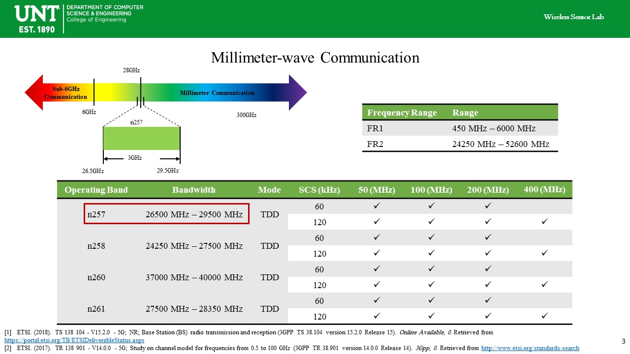 |
The millimeter-wave frequency range covers a frequency range between 6GHz and 300GHz. As most of you already know, the main idea behind using the millimeter-wave is to increase the network capacity by increasing the bandwidth. As you know, the sub-6GHz frequency ranges are highly congested. To access large bandwidth, we have to move to the higher frequencies. For example, the table shows that the n257 operating band provides an enormous bandwidth of 3GHz.
|
| ICACT20210129 Slide.04
[Big Slide]
|
Chrome Click!! |
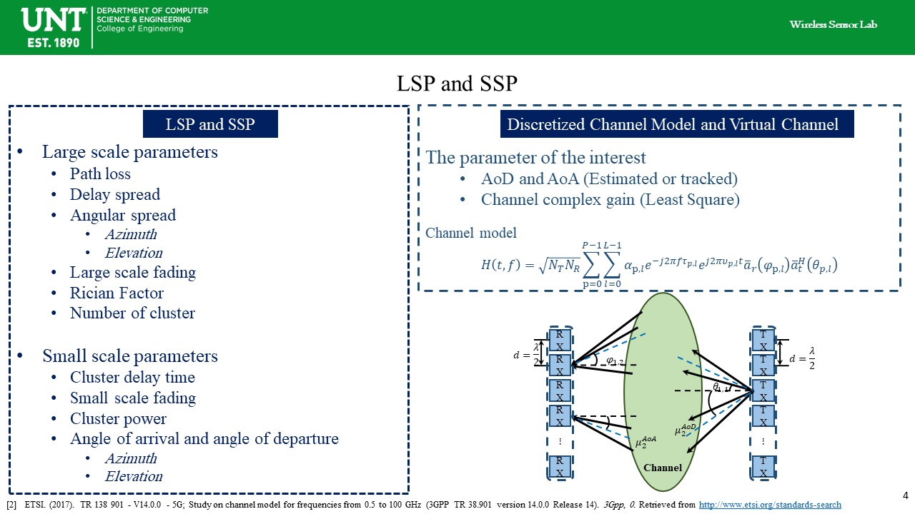 |
To understand millimeter-wave, we need to model the millimeter-wave channel properly to reflect its propagation characteristics. The large-scale behavior of the channel varies over longer distances, for example, in the order of a couple of meters. The large scale behavior is parameterized using the free-space path loss, delay spread of the channel, angular spread, etc. However, the communication between the transmitter and receiver takes place through multiple paths. And, the multiple paths will interfere constructively and destructively, also known as small-scale fading. To model multipath communication, each path is parameterized using small-scale parameters. The small-scale parameters we are using in this work are the azimuth angle of departure AoD, the azimuth angle of arrival AoA, and the complex gains. The channel transfer function as shown here is constructed using the delay and Doppler shift contribution of the paths, and the transmitter and receiver steering vectors formed using the angle of departure and angle of arrival. As a result, to identify the channel, one needs to estimate the small-scale parameters. Particularly, we are interested in estimating AoD, AoA, and complex channel gain.
|
| ICACT20210129 Slide.05
[Big Slide]
|
Chrome Click!! |
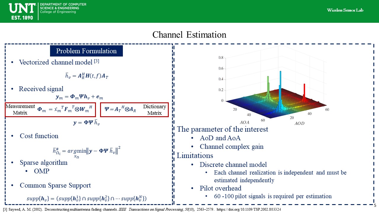 |
To estimate the channel parameters, we need to formulate the input-output relationship for the millimeter-wave system. Since the channel is sparse, the number of paths between the transmitter and receiver is much less than the channel dimension. One needs to formulate an input-output relationship in a sparse way. For this purpose, we need to use a sparse representation of the channel. The channel transfer matrix is mapped to its sparse unitary equivalent representation in the angular domain using the virtual channel model introduced by Sayeed. We formulate the received signal using the measurement matrix Phi and fixed dictionary matric Psi. This is a common formulation for millimeter-wave sparse communication. Then, we have a cost function formulated as a minimum square error. We are using Orthogonal Matching Pursuit for channel estimation. OMP is a fast greedy algorithm; since the estimation is not our primary focus in this paper, it satisfies the expectations. The figure here on the right shows example 64 by 64 sparse millimeter-wave channel with three paths. We can see that most of the matrix elements are zero, and there are few dominant components. We aim to estimate AoD and AoA using a minimum number of measurements. The state of the art measurements is shown to be about 60 to 100 for a 64 by 64 channel.
Because the channel transfer function is quantized, then one needs to transmit 60 to 100 pilot signals to estimate each channel realizations. This wastes the bandwidth and other resources.
|
| ICACT20210129 Slide.06
[Big Slide]
|
Chrome Click!! |
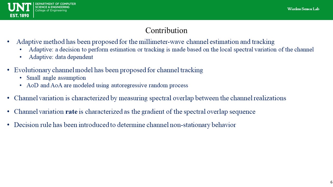 |
So, channel tracking's primary goal is to update the channel parameters instead of estimating each time and decrease the overall number of transmitted pilot signals. For this, one needs to consider the dynamics of the channel and how it varies with time. A couple of questions arise here. First, how can we measure the channel variation? Second, how to decide to select channel estimation or update channel parameters?
To answer the first question, we need to understand that the channel dynamics is characterized by the spectral overlap between the channel realizations. Moreover, the rate that the channel dynamics varies with time is measured statistically as the local spread of the spectral overlap between channel realizations.
We purpose to select channel estimation or channel tracking adaptively by characterizing the local dynamics of the channel. For this, we model the channel dynamics using its spectral properties. Then, locally, we decide if the channel experiences significant variation or not. If there is a significant channel variation, the channel parameters have to be estimated. Otherwise, they can be updated. To update the parameters, we purpose the evolutionary channel model using a small-angle assumption; that is, we assume the AoD and AoA are varying smoothly with time.
In the following slides, we discuss how to measure the spectral overlap between the channels and how to decide if the channel parameters have to be estimated or updated. |
| ICACT20210129 Slide.07
[Big Slide]
|
Chrome Click!! |
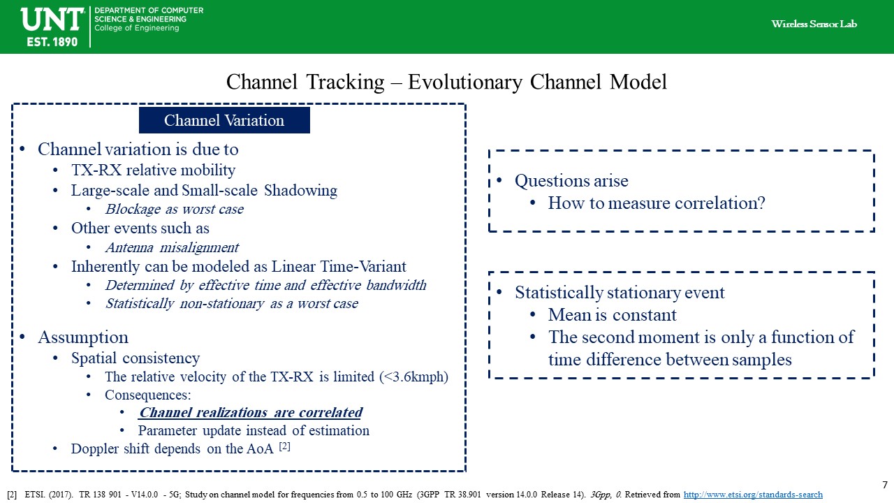 |
Channel varies with time because of several reasons—first, due to the receiver and transmitter mobility. Second, due to the artifacts such as antenna misalignment and, most importantly, shadowing and blockage. The best approach to model the time-variant channel is the linear time-variant model. By linearity, we make sure that the multiple communication paths are added up linearly. We also assume that the channel realizations are correlated under spatial consistency conditions. In spatial consistency mode, the transmitter and receiver relation speed is limited to less than 3.6kmph. The channel realizations that are measured close to each other temporally or spatially are correlated under spatial consistency. Moreover, we assume that the transmitter is fixed, and the Doppler shift is reflected on the AoA. By measuring the correlation order between the channels, we can measure the spectral overlap between the channels.
|
| ICACT20210129 Slide.08
[Big Slide]
|
Chrome Click!! |
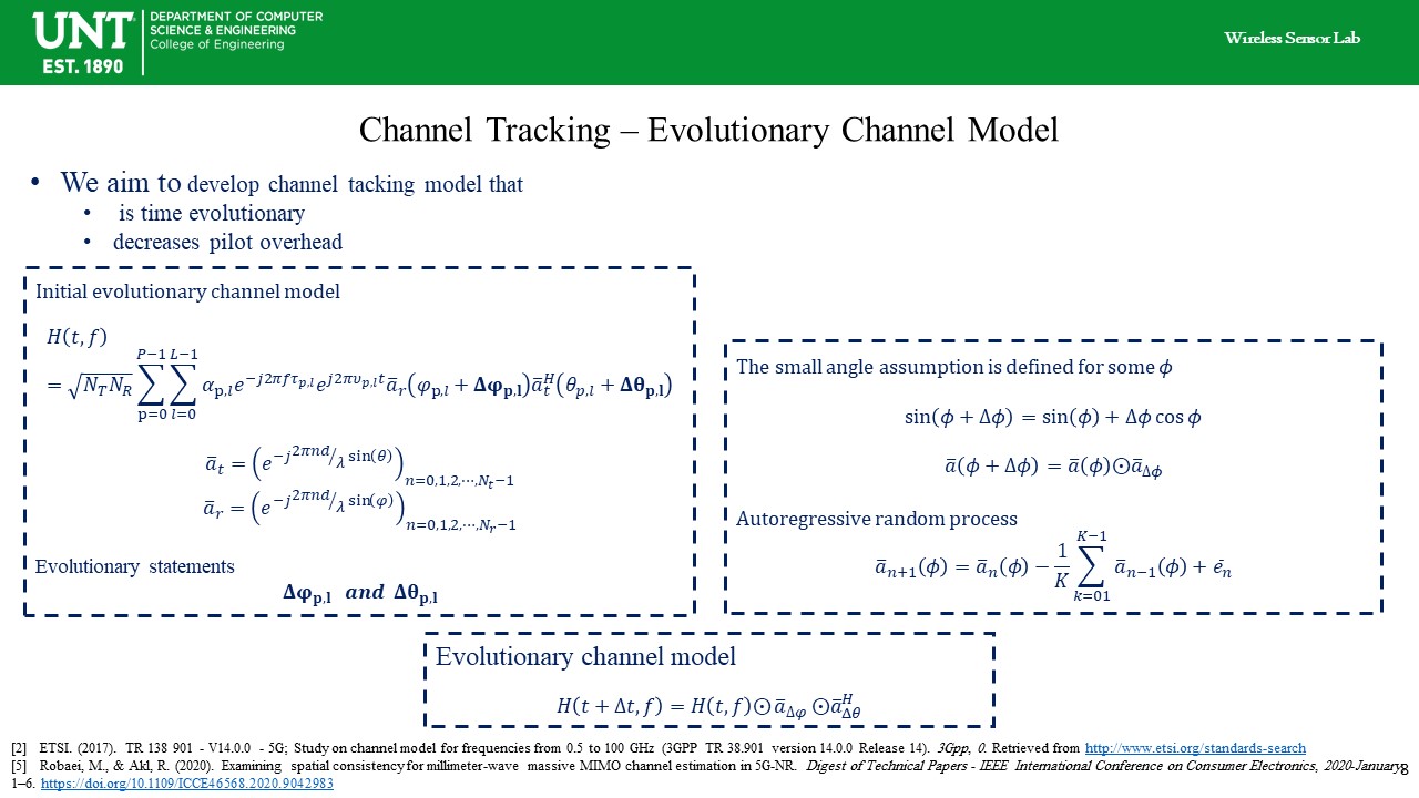 |
We have developed the evolutionary statement for the Saleh-Valenzuela by adding incremental statements delta phi and delta theta to the AoD and AoA, as is shown in the channel transfer function. We assume that the angular variations are small to substitute the sine and cosine with their small angle approximations. Since the AoD and AoA are best modeled using the random process, we model the angular variations using the autoregressive random process. In summary, the idea is to update the AoD and AoA as an autoregressive random process, then reconstruct the tracked channel using the evolutionary channel model. At time t plus delta t, the evolutionary channel can be represented as the Hadamard product of the channel transfer function at time t and the incremental steering vectors.
|
| ICACT20210129 Slide.09
[Big Slide]
|
Chrome Click!! |
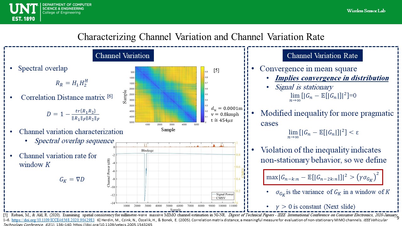 |
The correlation between channels can be measured using the correlation distance matrix recommended by Herdin et al. The correlation order determines the spectral overlap. The figure at the top shows the correlation for the 5000 channel realizations. As it is evident, the correlation disappears as the distance between the channels increases. We are also interested in how the spectral overlap varies with time. So, we create a sequence of the spectra overlaps. Then, we calculate the gradient of the spectral overlap sequence within some interval.
In order to detect the significant channel variation, we are using the convergence in mean square. It is known that the convergence in mean square implies convergence in the distribution. We use this idea to detect significant local channel variation. If the maximum value of convergence in mean square is greater than the local spread of the spectral overlap, then it means the local mean of the spectral overlap has been changes significantly. The maximum spread spectral overlap will be placed in the tail of the local distribution of the spectral overlap. As a result, its appearance increases the value of the convergence in mean square (because it is far from the mean).
This composes a decision rule for the adaptive channel estimation –tracking.
The figure at the bottom shows the blockage detected using the convergence in mean square. |
| ICACT20210129 Slide.10
[Big Slide]
|
Chrome Click!! |
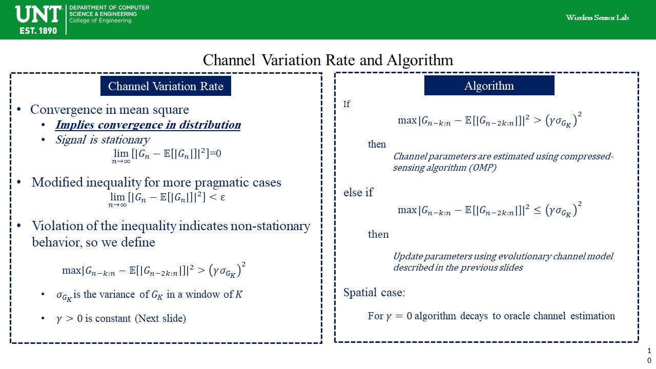 |
The algorithm is simple. We check the value returned by the convergence in mean square. If it is greater than the threshold, we estimate the channel parameter because updating parameters causes significant channel reconstruction error. Otherwise, the channel parameters are updated call channel tracking procedures. If the threshold is zero, then the algorithm decays to oracle channel estimation.
|
| ICACT20210129 Slide.11
[Big Slide]
|
Chrome Click!! |
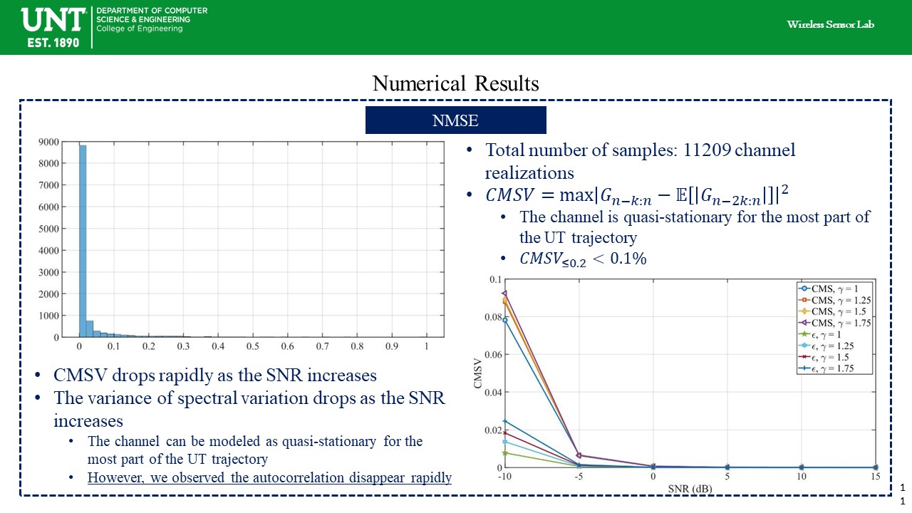 |
Let us look at how the channel varies with time. We collected 11209 channel realization over a 25 meters UT trajectory. To model non-stationary events, we used blockage that affects both the channel's large and small scale parameters. As we can see from the histogram, the value of the convergence in mean square is concentrated around zero. That means for the most part of the UT trajectory, the channel was mostly stationary or quasi-stationary. We notice that less than 0.01 percent of the channel realizations experience convergence in mean square value greater than 0.1. Also, the convergence in mean square values decreases as the SNR increases; that is, at higher SNR regions, the channel is experiencing a little variation. We should notice that the window size is small, so the variations are highly localized.
|
| ICACT20210129 Slide.12
[Big Slide]
|
Chrome Click!! |
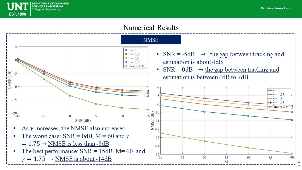 |
The normalized mean square error is an important parameter to evaluate the channel estimation and reconstruction error. As the SNR increases, the gap between the channel estimation error and channel tracking error increases. This is because as the SNR increases, the channel estimation becomes more and more accurate. Also, as the gamma increases, gamma was the constant to determines the threshold, the channel reconstruction error increases because more fluctuations are allowed during the channel tracking. The best result, negative 10dB NMSE, has been obtained for 90 measurements at 15dB SNR and gamma of 1.
|
| ICACT20210129 Slide.13
[Big Slide]
|
Chrome Click!! |
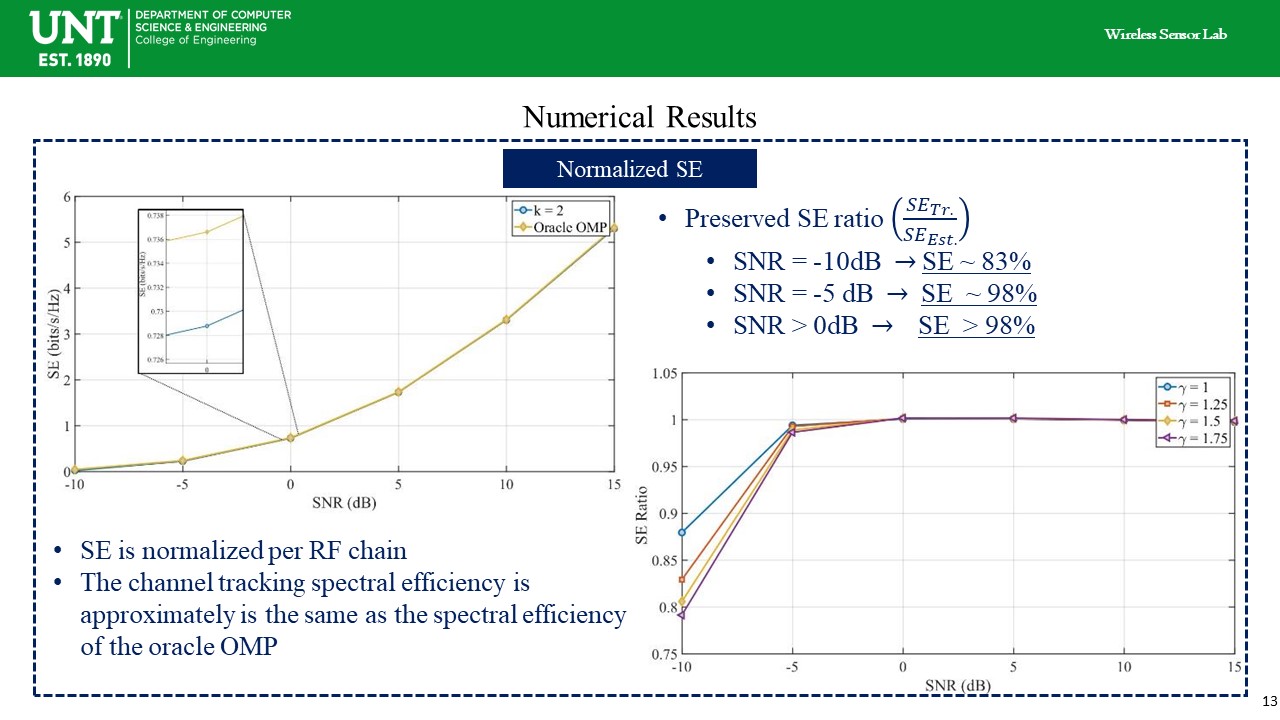 |
The spectral efficiency is the most critical criteria for network performance. It reflects how efficient a bandwidth has been used. We observe that at negative 10dB, the channel tracking preserves 83% of the spectral efficiency achieved by the oracle channel estimation. At 0dB, this is about 98%. This means that we can significantly relax the pilot requirement using channel tracking without sacrificing the spectral efficiency.
|
| ICACT20210129 Slide.14
[Big Slide]
|
Chrome Click!! |
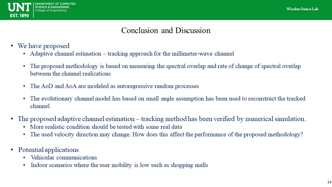 |
In summary, we discussed the adaptive channel estimation–tracking for millimeter-wave communication. We talked about the spectral overlap and its rate of change. We described how the spectral overlap is related to the channel dynamics through the correlation between the channel realizations. We examined the proposed method placing blockage randomly in the UT trajectory. However, this was only a synthetic condition. The proposed method should be tested using real data for a variety of conditions. The condition such as the user direction may change suddenly, or the user's velocity may change.
Finally, the potential applications are vehicular communication, indoor communication, and pedestrian users.
|
| ICACT20210129 Slide.15
[Big Slide]
|
Chrome Click!! |
 |
I want to thank Dr. Akl, the computer science and engineering department at the University of North Texas, the Toulouse grad school, and the UNT HPC center that provided high-performance computational facilities to run and collect data.
|
| ICACT20210129 Slide.16
[Big Slide]
|
Chrome Click!! |
 |
Thank you. Any questions?
|
| |