ICACT20210142 Slide.01
[Big Slide] |
Chrome  Click!! |
 |
Hello everyone, I am Dr. Munene Kanampiu. In this conference I am presenting the work of myself and my partner, Dr. Jinsuk Baek, both of us from the Winston-Salem state university, NC. USA. Today we present our work on a computational model for a strategic sensor placement for a smart farm water sprinkler system. |
| ICACT20210142 Slide.02
[Big Slide]
|
Chrome Click!! |
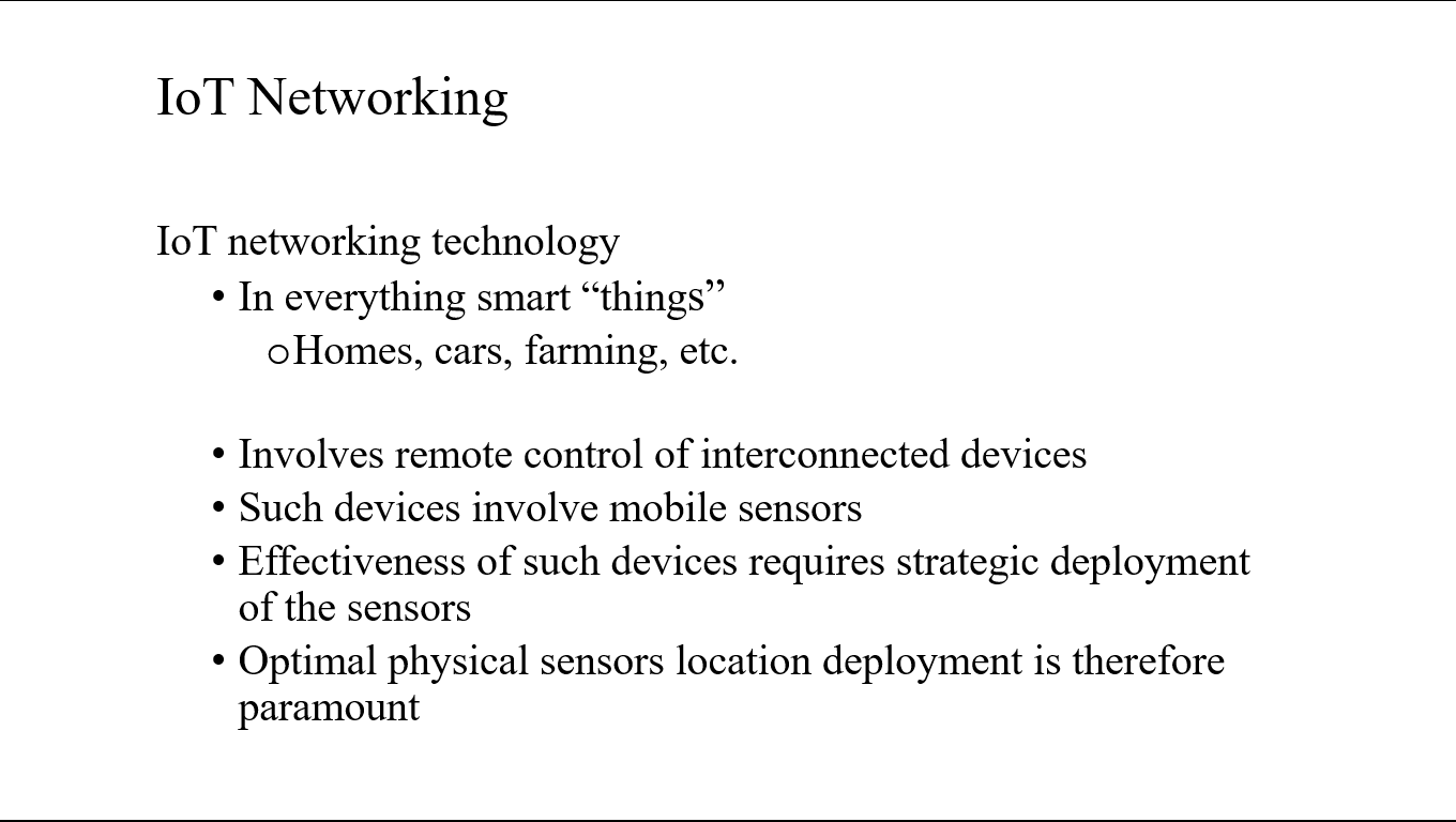 |
IoT networking technology is in everything smart “things” e.g., homes, cars, farming, etc.
It Involves remote control of interconnected devices that in themselves use mobile sensors.
Effectiveness of such devices requires strategic deployment of the sensors. As such optimal physical sensors’ location deployment is therefore paramount
|
| ICACT20210142 Slide.03
[Big Slide]
|
Chrome Click!! |
 |
Our work on developing an Optimal Sensor Placement computation model for a smart farm aims at optimizing the location of water sprinkler sensors for the farm to ensure minimal overlap coverage area……Even-spread with no un-watered patches |
| ICACT20210142 Slide.04
[Big Slide]
|
Chrome Click!! |
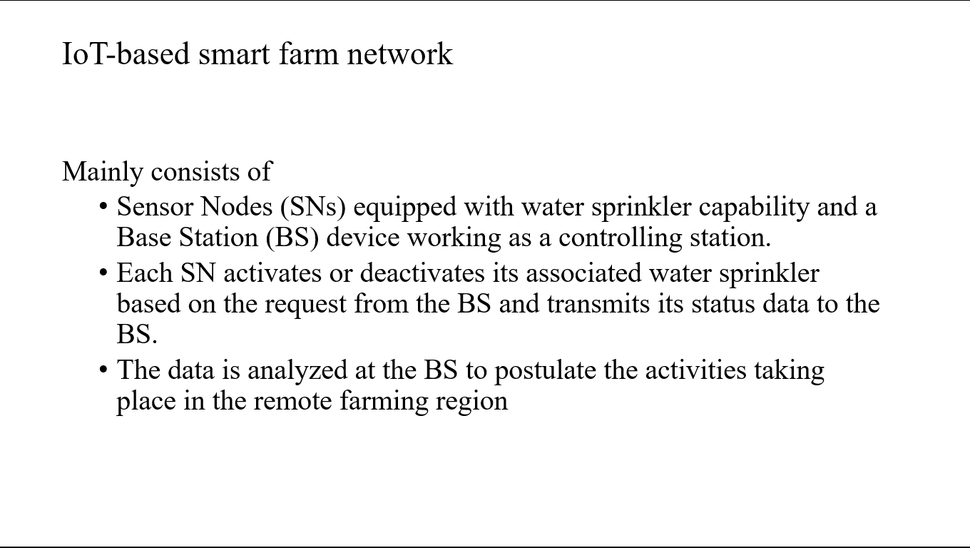 |
IoT-based smart farm network mainly consists of sensor nodes (SNs) equipped with water sprinkler capability and a base station (BS) device working as a controlling station. Each SN activates or deactivates its associated water sprinkler based on the request from the BS and transmits its status data to the BS. The data is analyzed at the BS to postulate the activities taking place in the remote farming region. |
| ICACT20210142 Slide.05
[Big Slide]
|
Chrome Click!! |
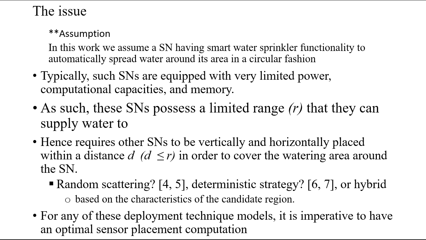 |
The issue is: such SNs are usually equipped with very limited power, computational capacities, and memory. As such, these SNs possess a limited range (r) that they can supply water to hence requires other SNs to be vertically and horizontally placed within a distance d (d ≤ r) in order to cover the watering area around the SN. These placement strategies include random scattering [4, 5], deterministic strategy [6, 7], or hybrid, based on the characteristics of the candidate region. For any of these deployment technique models, it is imperative to have an optimal sensor placement computation |
| ICACT20210142 Slide.06
[Big Slide]
|
Chrome Click!! |
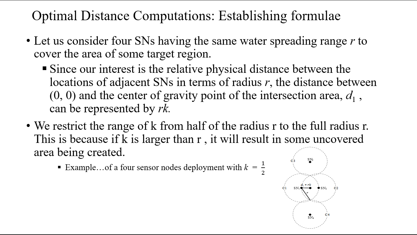 |
To establish the formula for the optimal distance computation, we consider four SNs having the same water spreading range r to cover the area of some target region.
Since our interest is the relative physical distance between the locations of adjacent SNs in terms of radius r, the distance between (0, 0) and the center of gravity point of the intersection area, d1 , can be represented by rk. We restrict the range of k from half of the radius r to the full radius r. This is because if k is larger than r, it will result in creation of some uncovered area
|
| ICACT20210142 Slide.07
[Big Slide]
|
Chrome Click!! |
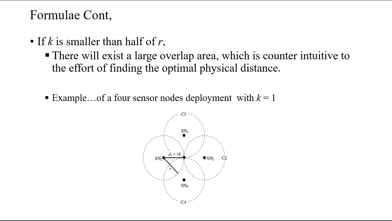 |
Likewise, if k is smaller than half of r, then there will exist a large overlap area, which is counter intuitive to the effort of finding the optimal physical distance. |
| ICACT20210142 Slide.08
[Big Slide]
|
Chrome Click!! |
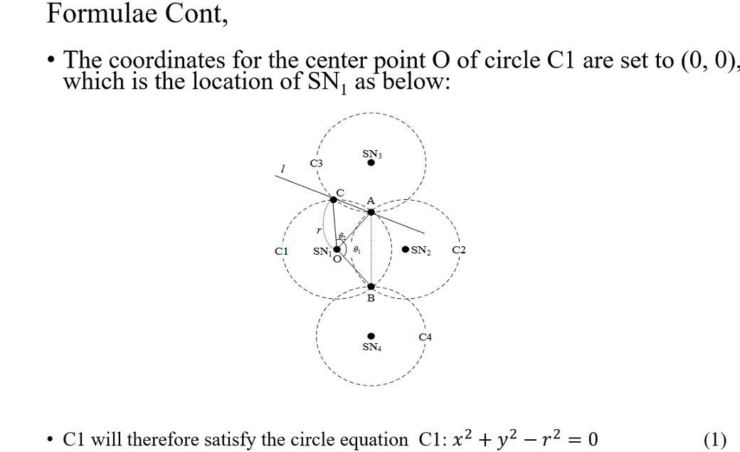 |
With the coordinates for the center point O of circle C1 set to (0, 0), which is the location of SN1
, C1 will therefore satisfy the circle equation: C1: x^2+y^2-r^2=0 ....... (1)
|
| ICACT20210142 Slide.09
[Big Slide]
|
Chrome Click!! |
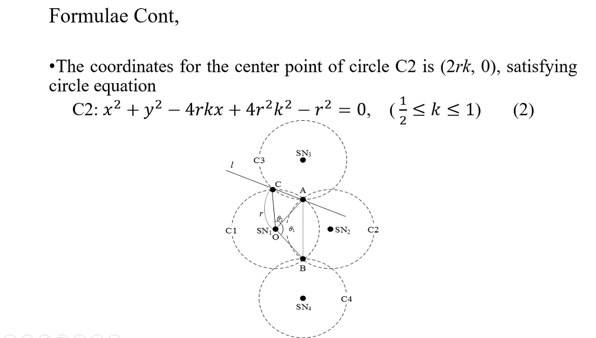 |
The coordinates for the center point of circle C2 are (2rk, 0), satisfying circle equation
C2: x^2+y^2-4rkx+4r^2 k^2-r^2=0, ( 1/2≤k≤1) ………….. (2)
|
| ICACT20210142 Slide.10
[Big Slide]
|
Chrome Click!! |
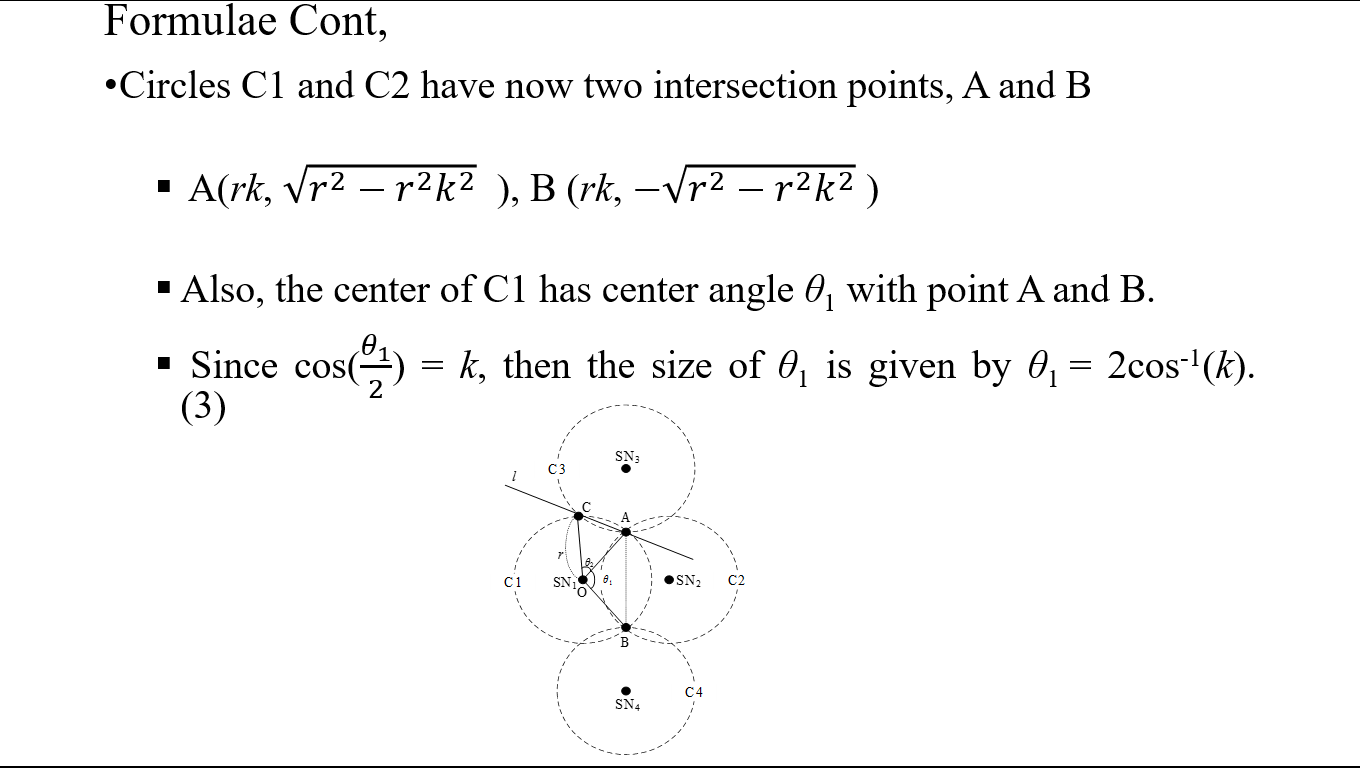 |
Circles C1 and C2 have now two intersection points, A and B, A(rk, √(r^2-〖r^2 k〗^2 ) ), B (rk, -√(r^2-〖r^2 k〗^2 ) ) . Also, the center of C1 has center angle θ1 with point A and B.
Since cos(θ_1/2) = k, then the size of θ1 is given by θ1 = 2cos-1(k). …………………… (3)
|
| ICACT20210142 Slide.11
[Big Slide]
|
Chrome Click!! |
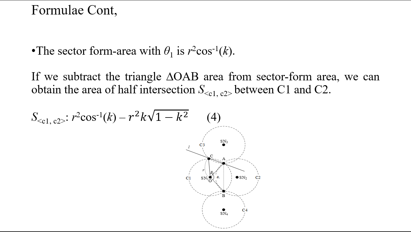 |
The sector form-area with θ1 is r2cos-1(k). By subtracting the triangle ∆OAB area from sector-form area, we can obtain the area of half intersection S between C1 and C2. S: r2cos-1(k) – r^2 k√(1-k^2 ) ……. (4) |
| ICACT20210142 Slide.12
[Big Slide]
|
Chrome Click!! |
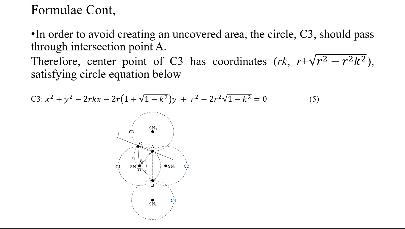 |
To avoid creating an uncovered area, the circle, C3, should pass through intersection point A.
Therefore, center point of C3 has coordinates (rk, r+√(r^2-〖r^2 k〗^2 )), satisfying circle equation
C3: x^2+y^2-2rkx-2r(1+√(1-k^2 ))y + r^2+〖2r〗^2 √(1-k^2 )=0 ………….. (5)
|
| ICACT20210142 Slide.13
[Big Slide]
|
Chrome Click!! |
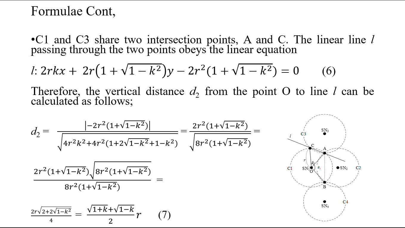 |
C1 and C3 share two intersection points, A and C. The linear line l passing through the two points obeys the linear equation
l: 2rkx+ 2r(1+√(1-k^2 ))y-〖2r〗^2 (1+√(1-k^2 ))=0 ....... (6)
Therefore, the vertical distance d2 from the point O to line l can be calculated as follows;
d2 = |-〖2r〗^2 (1+√(1-k^2 ))|/√(4r^2 k^2+4r^2 (1+2√(1-k^2 )+1-k^2)) = (〖2r〗^2 (1+√(1-k^2 )))/√(8r^2 (1+√(1-k^2 ))) = (〖2r〗^2 (1+√(1-k^2 ))√(8r^2 (1+√(1-k^2 ))))/(8r^2 (1+√(1-k^2 ))) =(2r√(2+2√(1-k^2 )) )/4 =
(√(1+k)+√(1-k))/2 r ...................... (7)
|
| ICACT20210142 Slide.14
[Big Slide]
|
Chrome Click!! |
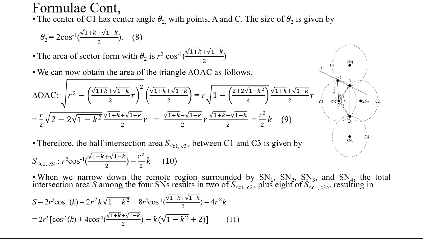 |
The center of C1 has center angle θ2, with points, A and C.
The size of θ2 is given by θ2 = 2cos-1((√(1+k)+√(1-k))/2)....(8)
The area of sector-form with θ2 is r2 cos-1((√(1+k)+√(1-k))/2)
We can now obtain the area of the triangle ∆OAC as follows:
∆OAC: √(r^2-((√(1+k)+√(1-k))/2 r)^2 ) ((√(1+k)+√(1-k))/2) = r√(1-((2+2√(1-k^2 ))/4) ) (√(1+k)+√(1-k))/2 r =
r/2 √(2-2√(1-k^2 (√(1+k)+√(1-k))/2 r = (√(1+k)-√(1-k))/2 r (√(1+k)+√(1-k))/2 = r^2/2 k …………….. (9)
Therefore, the half intersection area S between C1 and C3 is given by S: r2cos-1((√(1+k)+√(1-k))/2) – r^2/2 k ………. (10).
When we narrow down the remote region surrounded by SN1, SN2, SN3, and SN4, the total intersection area S among the four SNs results in two of S plus eight of S, resulting in S = 2r2cos-1(k) – 2r^2 k√(1-k^2 ) + 8r2cos-1((√(1+k)+√(1-k))/2) – 4r^2 k = 2r2 [cos-1(k) + 4cos-1((√(1+k)+√(1-k))/2)-k(√(1-k^2 )+2)] . .. . ....(11)
|
| ICACT20210142 Slide.15
[Big Slide]
|
Chrome Click!! |
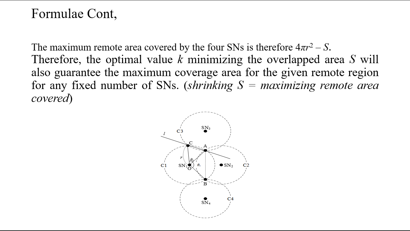 |
The maximum remote area covered by the four SNs is therefore 4πr2 – S.
As such, the optimal value k minimizing the overlapped area S will also guarantee the maximum coverage area for the given remote region for any fixed number of SNs. (shrinking S = maximizing remote area covered)
|
| ICACT20210142 Slide.16
[Big Slide]
|
Chrome Click!! |
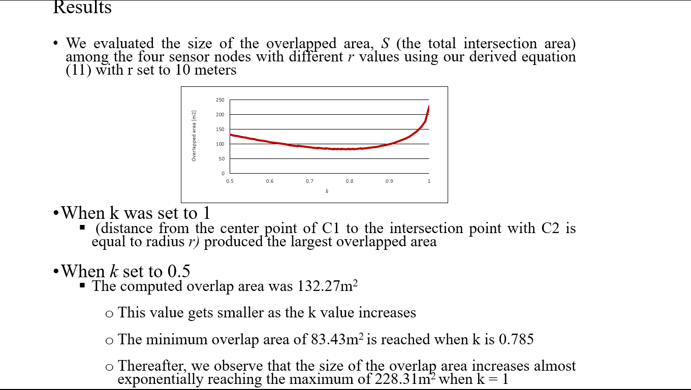 |
We evaluated the size of the overlapped area, S (the total intersection area) among the four sensor nodes with different r values using our derived equation (11) with r set to 10 meters. When k was set to 1 (distance from the center point of C1 to the intersection point with C2 is equal to radius r) produced the largest overlapped area. When k set to 0.5, the computed overlap area was 132.27m2. This value gets smaller as the k value increases. The minimum overlap area of 83.43m2 is reached when k is 0.785. Thereafter, we observe that the size of the overlap area increases almost exponentially reaching the maximum of 228.31m2 when k = 1 |
| ICACT20210142 Slide.17
[Big Slide]
|
Chrome Click!! |
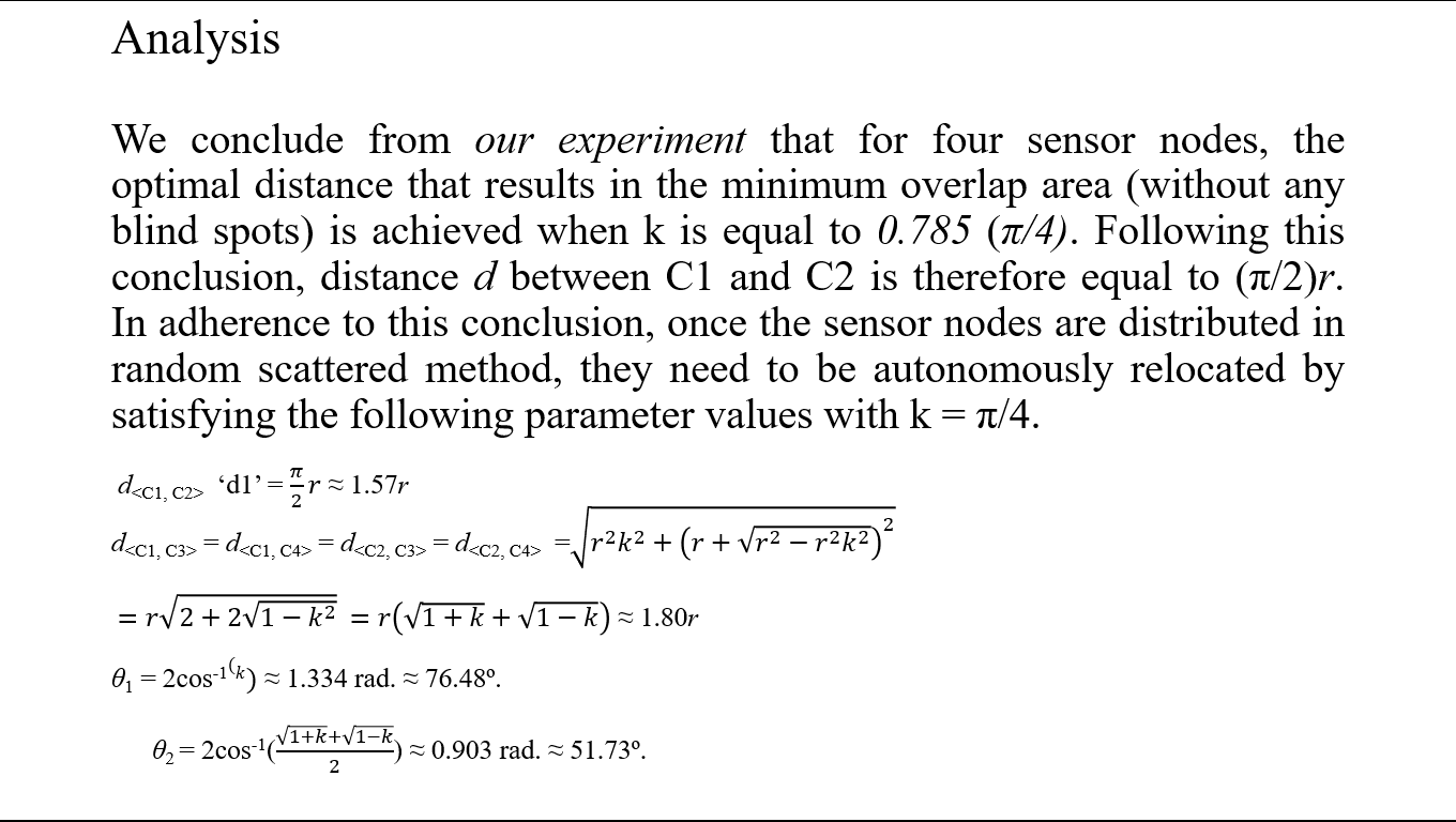 |
Based on our experiment we concluded that for four sensor nodes, the optimal distance that results in the minimum overlap area (without any blind spots) is achieved when k is equal to 0.785 (π/4). Following this conclusion, distance d between C1 and C2 is therefore equal to (π/2)r. In adherence to this conclusion, once the sensor nodes are distributed in random scattered method, they need to be autonomously relocated by satisfying the following parameter values with k = π/4:
d: ‘d1’ = π/2 r ≈ 1.57r
d = d = d = d = √(r^2 k^2+(r+√(r^2-r^2 k^2 ))^2 ) =r√(2+2√(1-k^2 )) =
r(√(1+k)+√(1-k)) ≈ 1.80r
θ1 = 2cos-1(k) ≈ 1.334 rad. ≈ 76.48º.
θ2 = 2cos-1((√(1+k)+√(1-k))/2) ≈ 0.903 rad. ≈ 51.73º
|
| ICACT20210142 Slide.18
[Big Slide]
|
Chrome Click!! |
 |
We compared the number of sensors required to cover the area of a given circular target of radius R using the optimized computation parameter values for sensor deployment and using the well-aligned but NOT optimized sensor deployment. To do this we imagined a target farming area divided into grids and designated each sensor to cover a grid. Since the area of each grid should be fully covered by a sensor, its area should intuitively be less than the total area covered by the sensor. |
| ICACT20210142 Slide.19
[Big Slide]
|
Chrome Click!! |
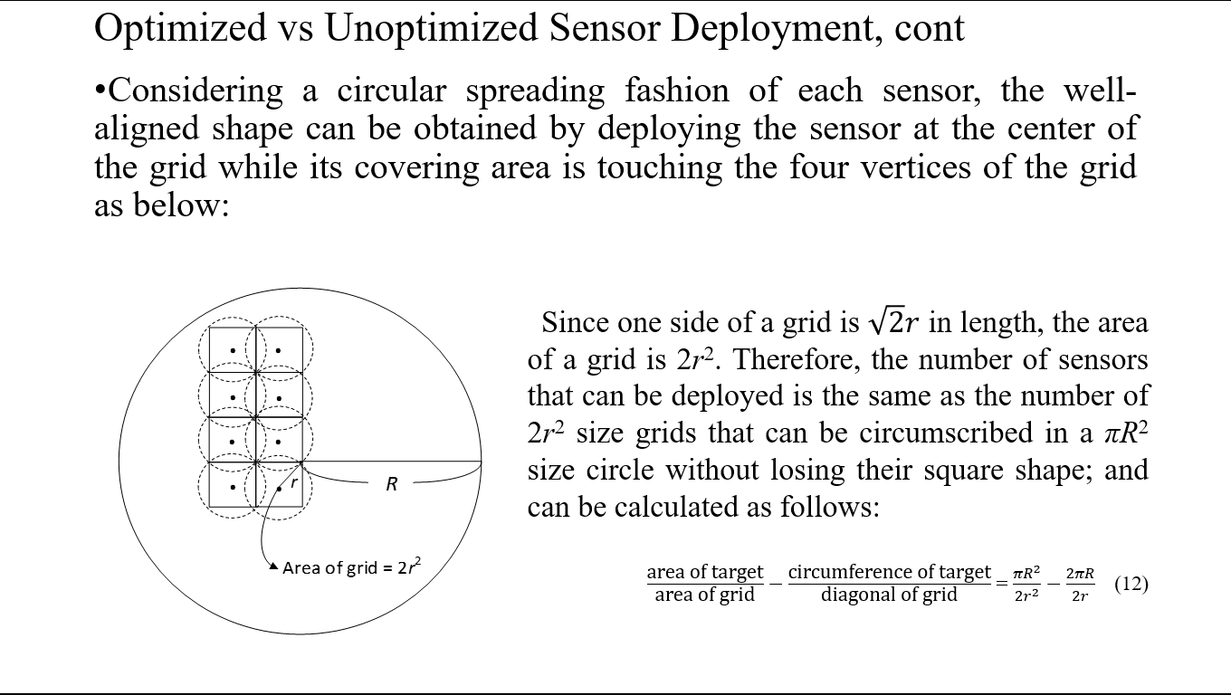 |
Considering a circular spreading fashion of each sensor, the well-aligned shape can be obtained by deploying the sensor at the center of the grid while its covering area is touching the four vertices of the grid: Since one side of a grid is √2 r in length, the area of a grid is 2r2. Therefore, the number of sensors that can be deployed is the same as the number of 2r2 size grids that can be circumscribed in a πR2 size circle without losing their square shape; and can be calculated as follows:
"area of target" /"area of grid" -"circumference of target" /"diagonal of grid" = (πR^2)/(2r^2 )-2πR/2r …… (12)
|
| ICACT20210142 Slide.20
[Big Slide]
|
Chrome Click!! |
 |
As such, the most important factor in deciding the number of sensors required to fully cover a given target area is the grid size. For our optimized sensor deployment, the shape of the grid is not square but rectangular. The grid width is given by 2rk |
| ICACT20210142 Slide.21
[Big Slide]
|
Chrome Click!! |
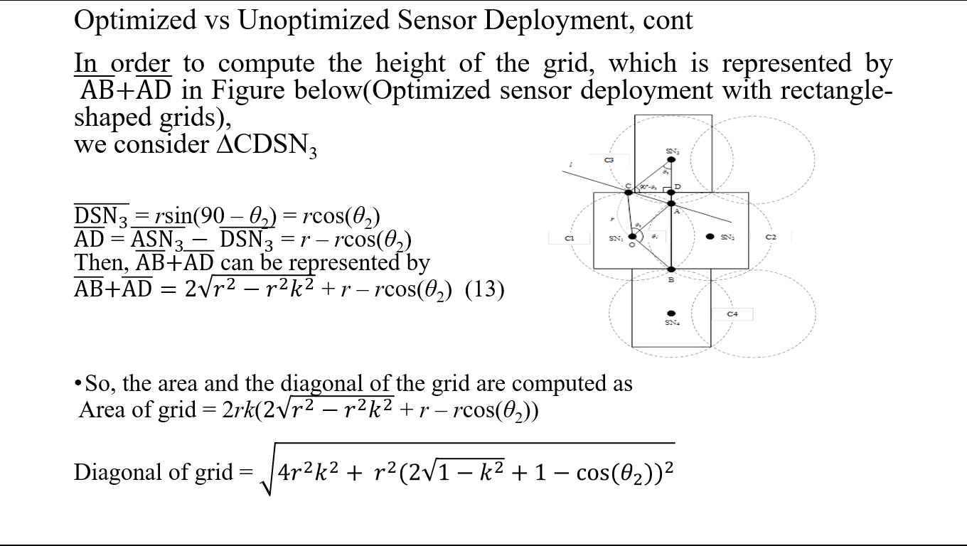 |
In order to compute the height of the grid, which is represented by AB + AD (Optimized sensor deployment with rectangle-shaped grids), we consider ∆CDSN_3 .
line DSN_3 = rsin(90 – θ2) = rcos(θ2)
Line AD = Line ASN_3 - line DSN_3 = r – rcos(θ2)
So, lines BA + AD can be represented by lines AB +AD =
2√(r^2-〖r^2 k〗^2 ) + r – rcos(θ2) ………… (13)
Therefore, the area and the diagonal of the grid are computed as follows:
Area of grid = 2rk(2√(r^2-〖r^2 k〗^2 ) + r – rcos(θ2))
Diagonal of grid = √(4〖r^2 k〗^2+ 〖r^2 (2√(1-k^2 )+1-cos(θ_2))〗^2 )
|
| ICACT20210142 Slide.22
[Big Slide]
|
Chrome Click!! |
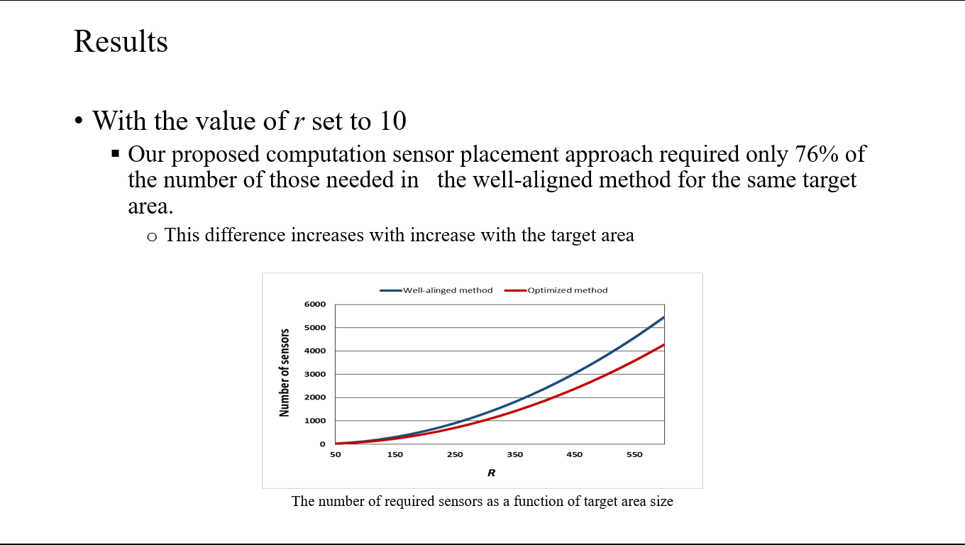 |
With the value of r set to 10, our proposed computation sensor placement approach required only 76% of the number of those needed in the well-aligned method for the same target area. This difference increases with increase with the target area |
| ICACT20210142 Slide.23
[Big Slide]
|
Chrome Click!! |
 |
Our proposed sprinkler sensors positioning based on our computational model ensures minimum overlap coverage area while at the same time ensuring that no area in the target zone is left uncovered.
The limitations are that we assumed a flat, even, and unobstructed region, applicable only in limited small-sized and controlled farming areas. It is therefore not applicable in uneven/physical obstructions areas. We will improve our work by extending the approach to a more robust 3D framework applicable in the real world: a real world of physical man-made obstructions and natural undulating topologies
|
| ICACT20210142 Slide.24
[Big Slide]
|
Chrome Click!! |
 |
Thank you for your attention!
Floor open for comments.
|