ICACT20210153 Slide.01
[Big Slide]
[YouTube] |
Chrome  Click!! |
 |
Hello everyone and welcome to this presentation. I am Mi Tian, graduate student in the University of Victoria, Canada.
In the next 10 minutes I shall discuss techniques to build a Massive Multiple-Input Multiple-Output (MIMO, for short) base station.
In particular, these techniques are based on coarsely quantized measurements and fixed-point arithmetic.
I hope you will find it interesting.
|
| ICACT20210153 Slide.02
[Big Slide]
|
Chrome Click!! |
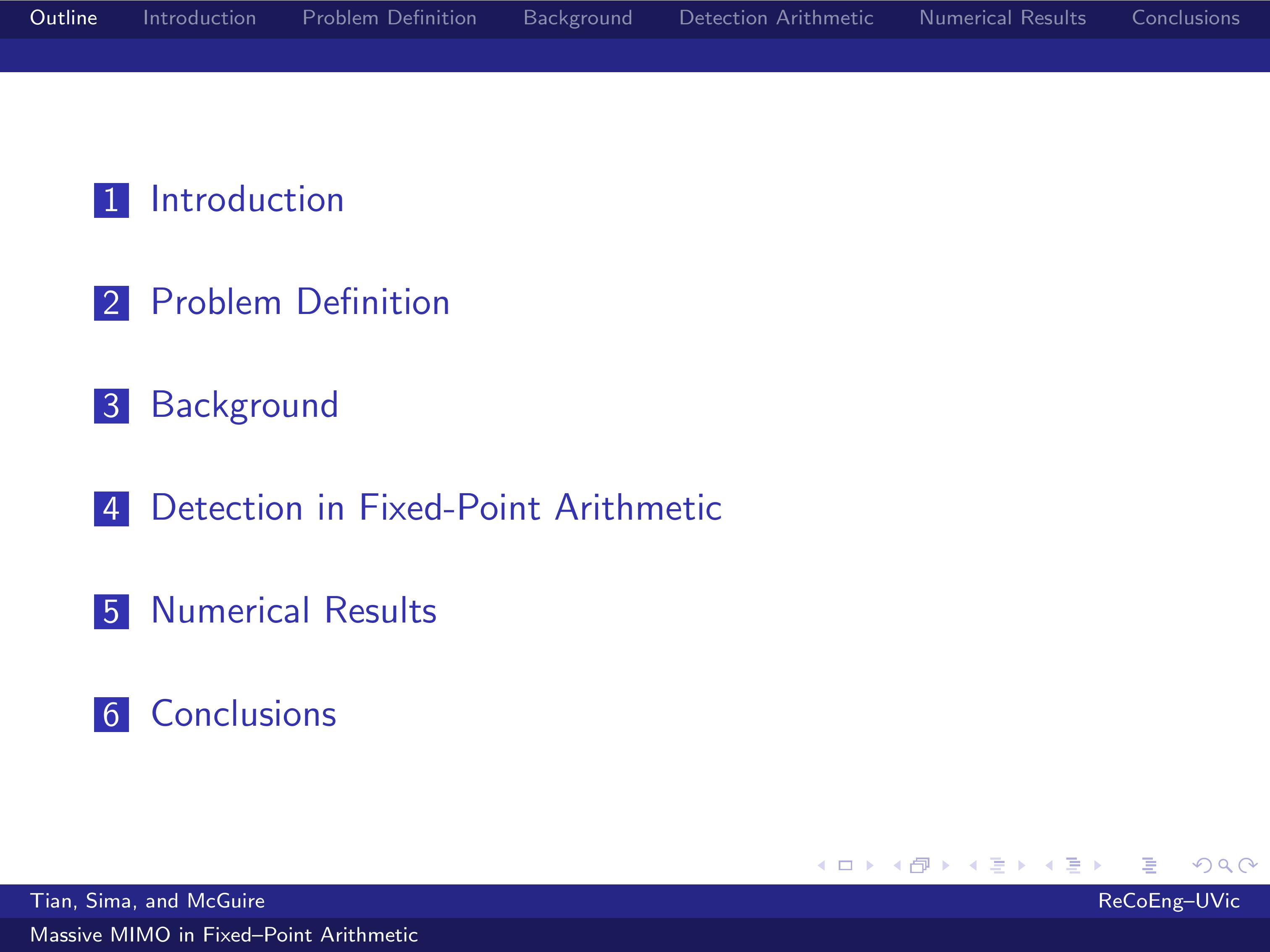 |
My talk starts with an Introduction on Massive MIMO base stations.
Problem Definition will highlight the difficulties we encounter in building such Massive MIMO base stations.
Background information on iterative channel estimation and coarse quantization is next provided.
Detection in Fixed-Point Arithmetic is described and Numerical Results are provided.
The Conclusions section will complete this presentation.
|
| ICACT20210153 Slide.03
[Big Slide]
|
Chrome Click!! |
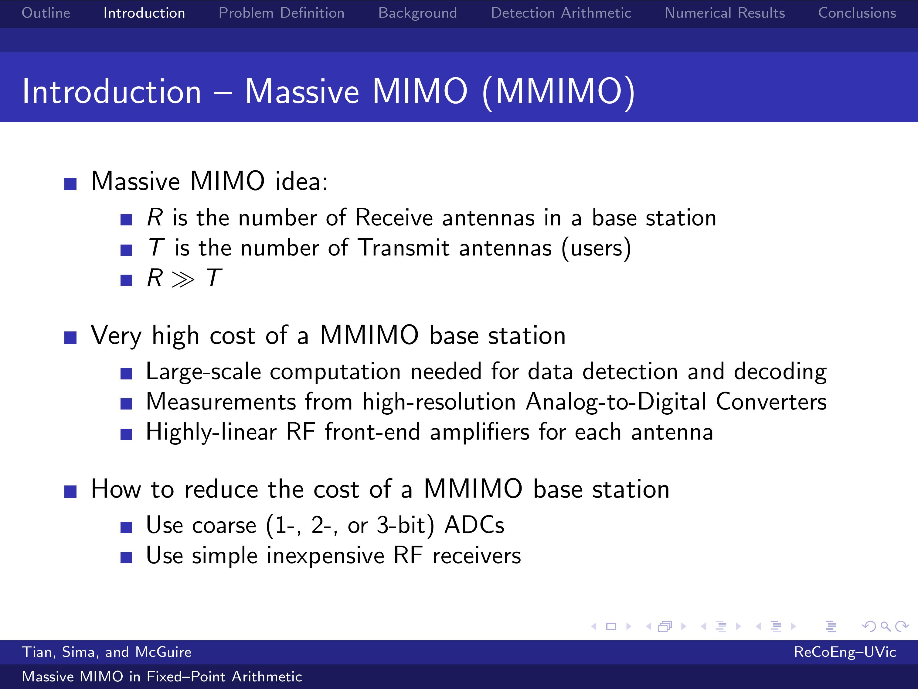 |
In a massive MIMO base station the number of Receive Antennas, R, is much larger than the number of Transmit Antennas, T, where we will consider one Transmit Antenna per User in this presentation.
Please observe that the cost of a Massive MIMO base station is very high, since large-scale computation is needed for data detection and decoding based on measurements from high-resolution Analog-to-Digital Converters, which are connected to highly linear RF front-end amplifiers for each Receive Antenna.
A way to reduce the cost of the implementation is to build the base stations with inexpensive low-end hardware, such as simple RF receivers feeding the received signals to coarse (1-, 2-, or 3-bit) Analog-to-Digital Converters.
|
| ICACT20210153 Slide.04
[Big Slide]
|
Chrome Click!! |
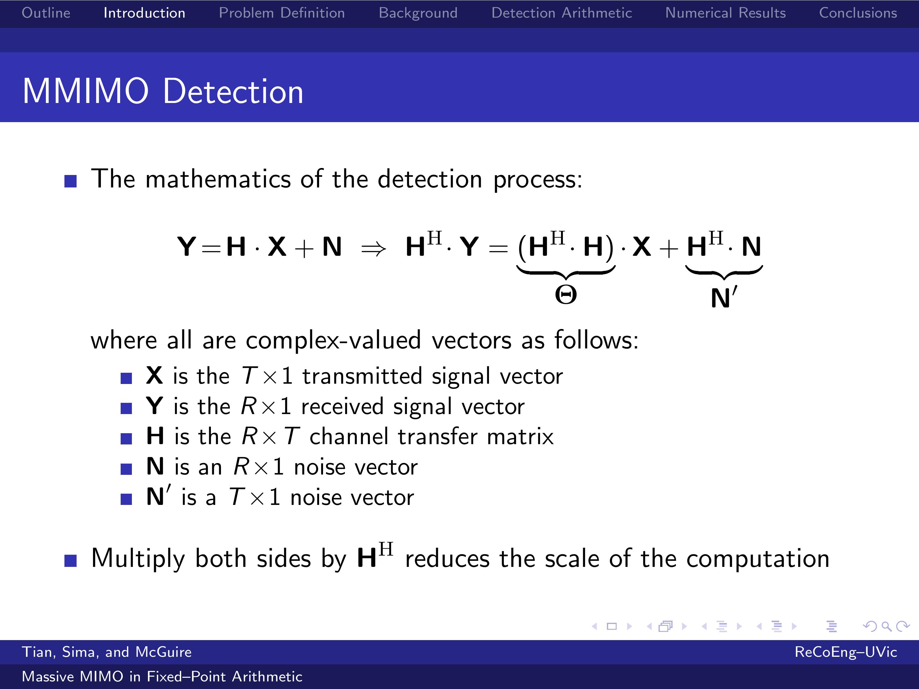 |
This slide shows the equation of the detection process, where X is the transmitted signal vector, Y is the received signal vector, H is the channel transfer matrix, N and N' are complex noise vectors.
With respect to this equation, please observe that the multiplication of both sides by H Hermitian transpose converts the R-by-T system to a T-by-T system, which is less expensive to solve.
The estimation of X through the solution of this linear system is the most computationally demanding portion of the receiver algorithm for reasonably high values of T.
|
| ICACT20210153 Slide.05
[Big Slide]
|
Chrome Click!! |
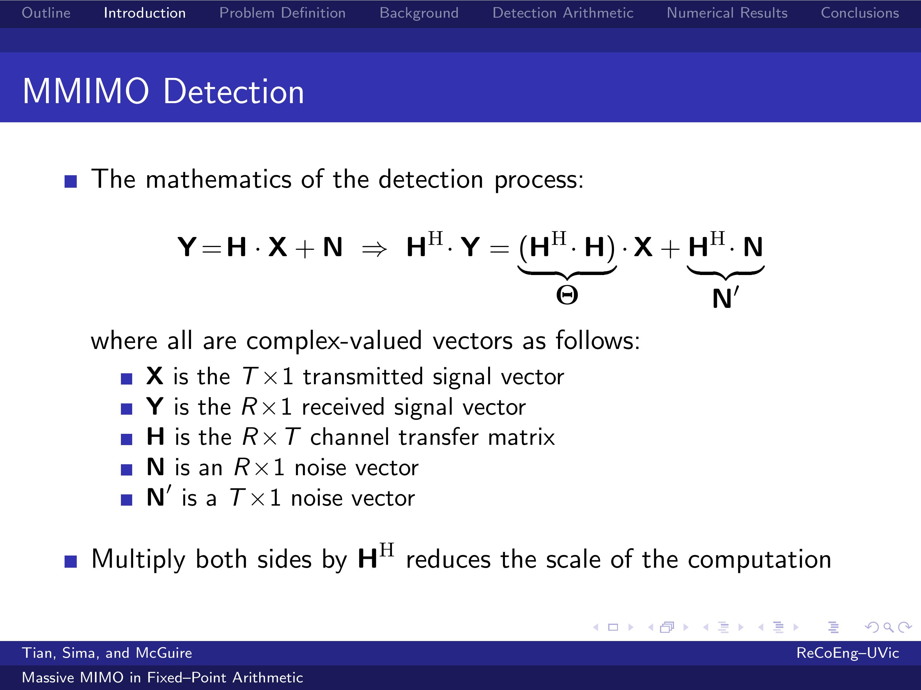 |
In this process, the following operations need to be performed: Calculation of the Hermitian matrix Theta, EigenValue Decomposition of matrix Theta, and Solving the linear system by matrix multiplications.
The challenge here is to perform these linear algebra operations in real time and with sufficient accuracy in order to achieve a good Bit-Error Rate.
That being said, I am now moving on to Problem Definition. |
| ICACT20210153 Slide.06
[Big Slide]
|
Chrome Click!! |
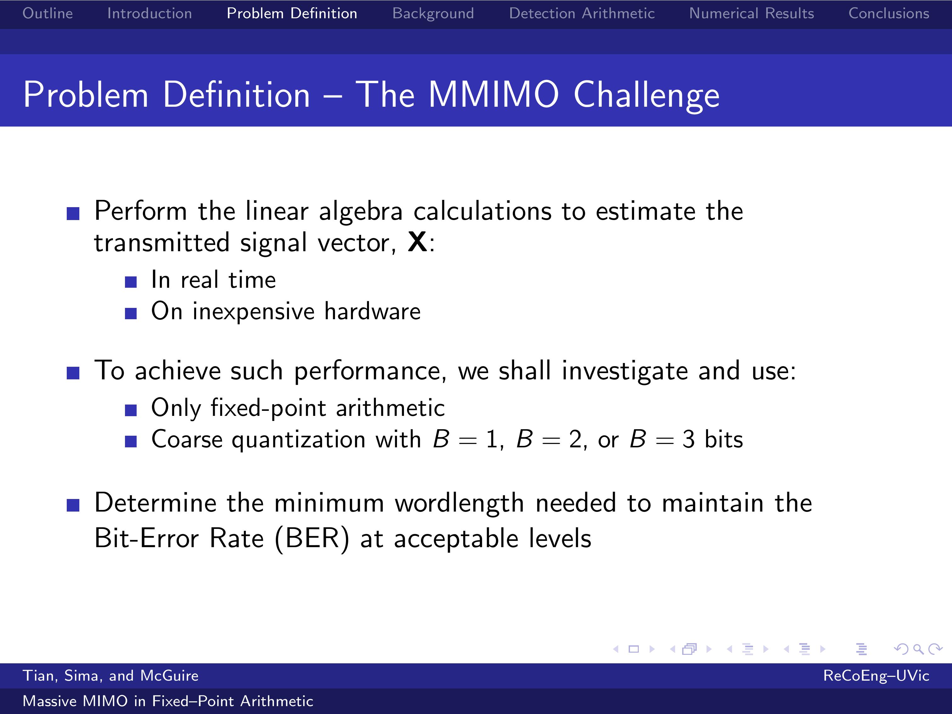 |
The big challenge in building a Massive MIMO base station is to perform the linear algebra calculations needed to estimate the transmitted signal vector, X, in real time on inexpensive hardware
In order to achieve such performance, we investigated and used only fixed-point arithmetic and coarse quantization with B=1, B=2, or B=3 quantization bits.
In our investigation, we aimed to determine the minimum wordlength needed to maintain the Bit-Error Rate at acceptable levels. |
| ICACT20210153 Slide.07
[Big Slide]
|
Chrome Click!! |
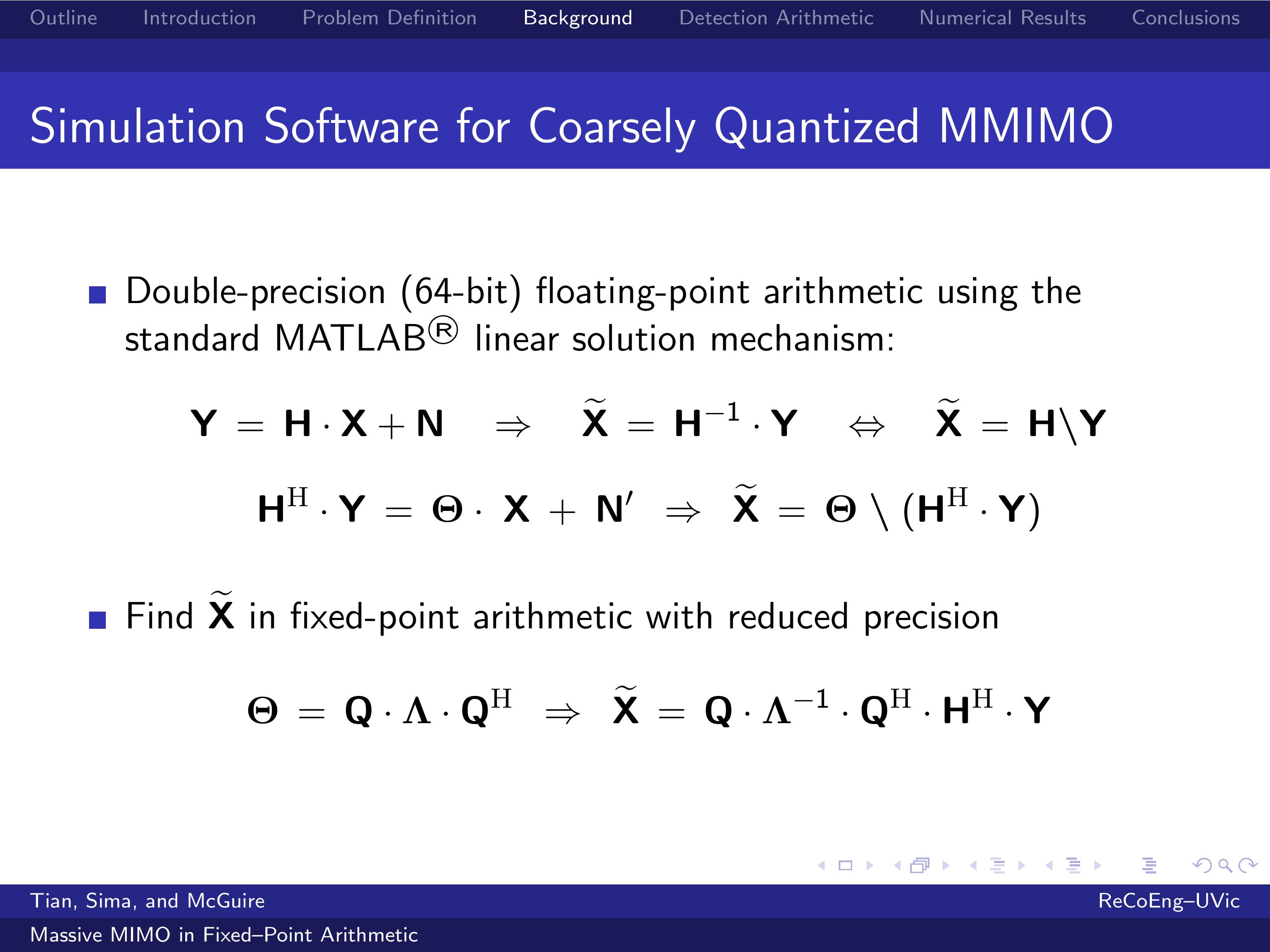 |
In our previous work, the linear system was solved in 64-bit floating-point arithmetic using the standard MATLAB linear solution mechanism, where X tilde = H inverse times Y is coded with the backslash operator, you can see in the first equation.
While these standard linear system solution computations give accurate results, direct implementation of these solutions for use in Massive MIMO receivers would require computational hardware with prohibitive cost in base stations.
To reduce the latency of estimating X, the linear system is solved in fixed-point arithmetic with reduced precision through an eigenvalue decomposition of the Hermitian matrix Theta. |
| ICACT20210153 Slide.08
[Big Slide]
|
Chrome Click!! |
 |
This slide presents issues related to coarse quantization.
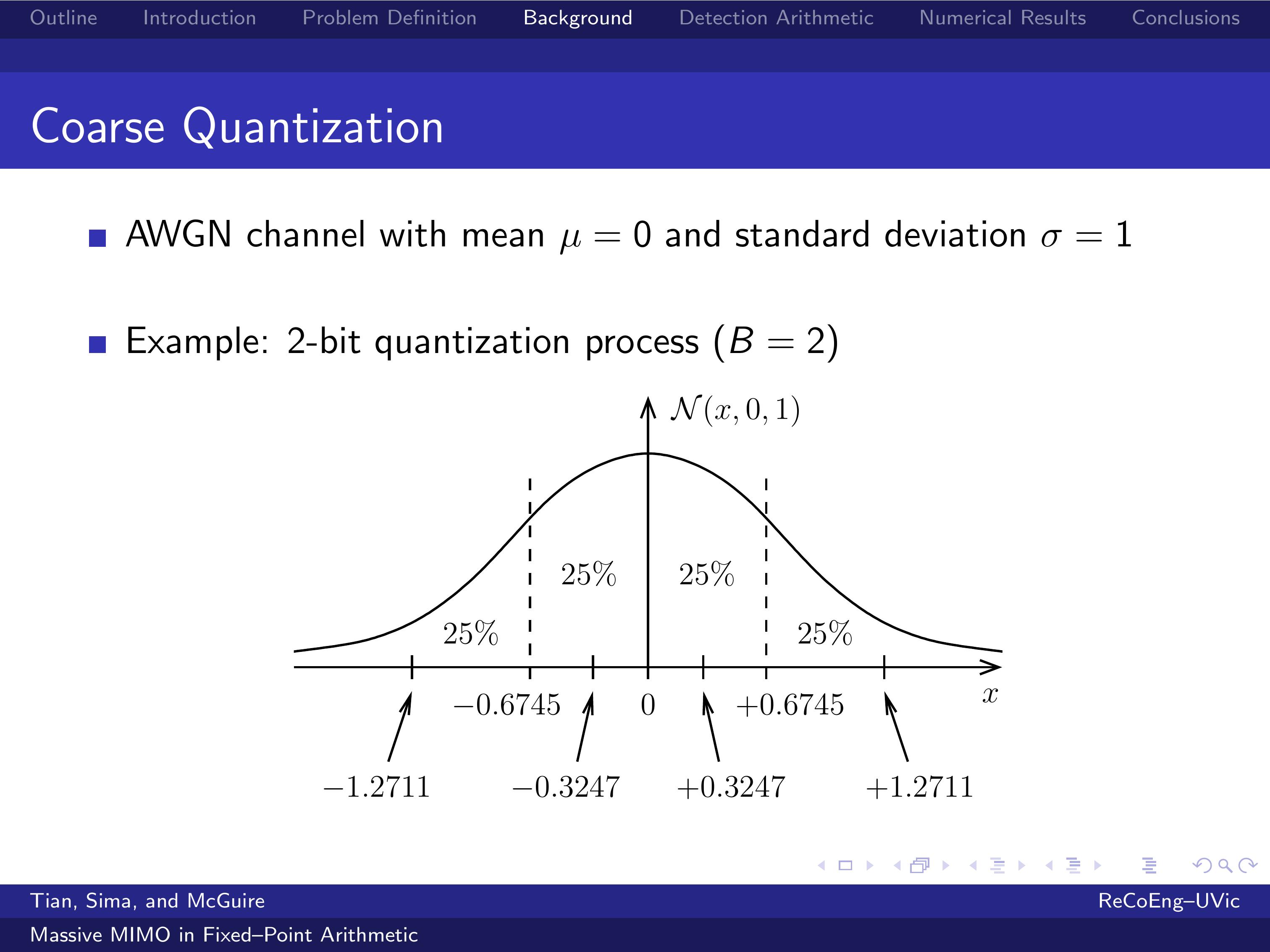
Please notice that an independent Additive White Gaussian Noise channel with mean zero and standard deviation 1 is assumed for each receive antenna.
The figure exemplifies a 2-bit quantization process which generates four quantization bins of equal probability (25%).
It can be easily calculated that the quantization thresholds are 0 and plus minus 0.6745, and the corresponding four bin-average values are plus minus 0.3247 and plus minus 1.2711. |
| ICACT20210153 Slide.09
[Big Slide]
|
Chrome Click!! |
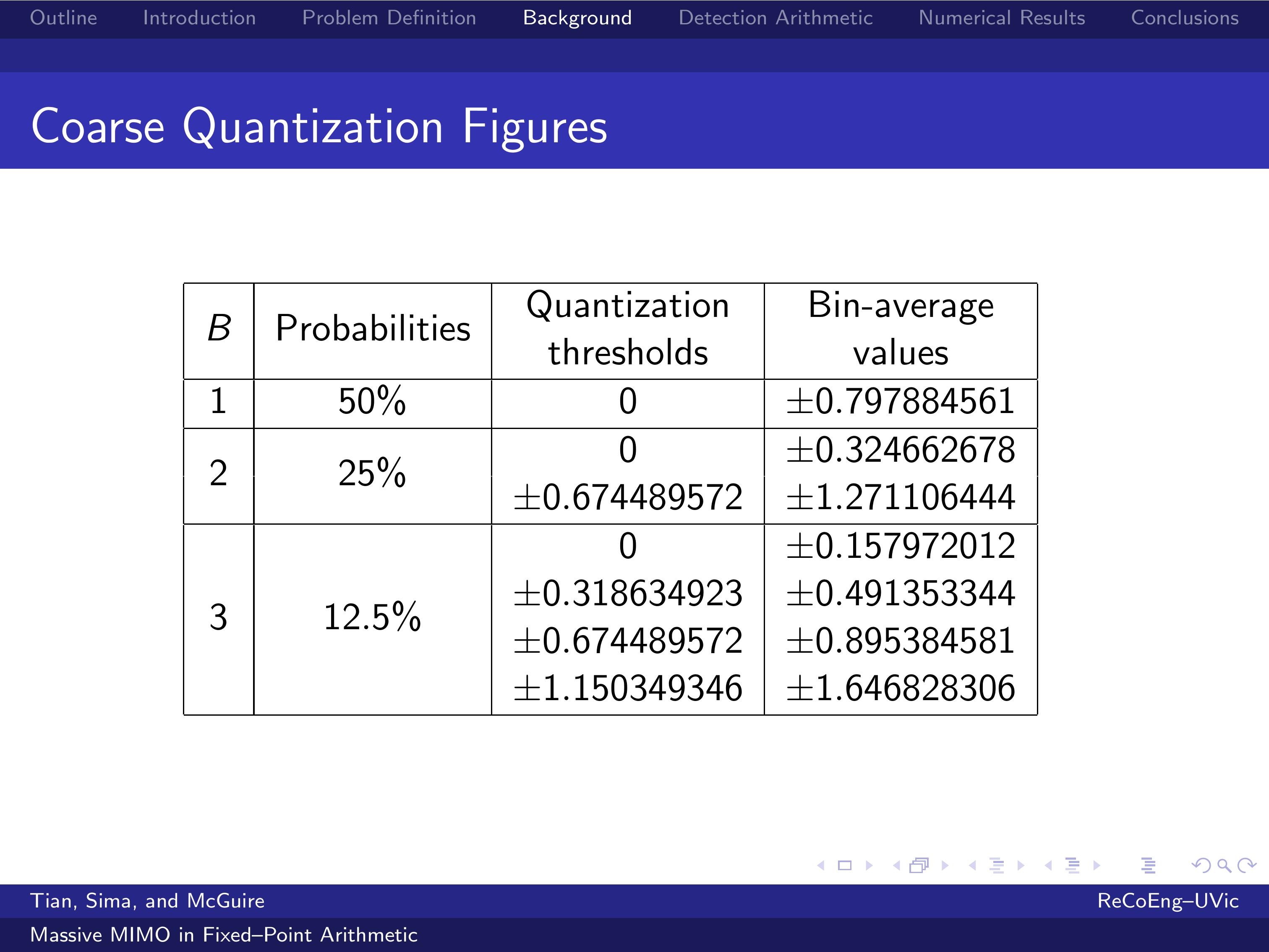 |
The table shows the probabilities, quantization thresholds, and the corresponding bin-average values for 1-bit, 2-bit, and 3-bit quantization processes for a Gaussian random variable with zero mean and unity standard deviation.
In fixed-point representation, it is beneficial to scale up the smallest magnitude of the bin-average values, since this will simplify the implementation and slightly increase the precision.
For example, in a 2-bit quantization process, 0.32 is promoted to 1.00, and 1.27 is promoted to 1.27 over 0.32, whish is 3.91.
The other quantization processes will follow a similar pattern.
|
| ICACT20210153 Slide.10
[Big Slide]
|
Chrome Click!! |
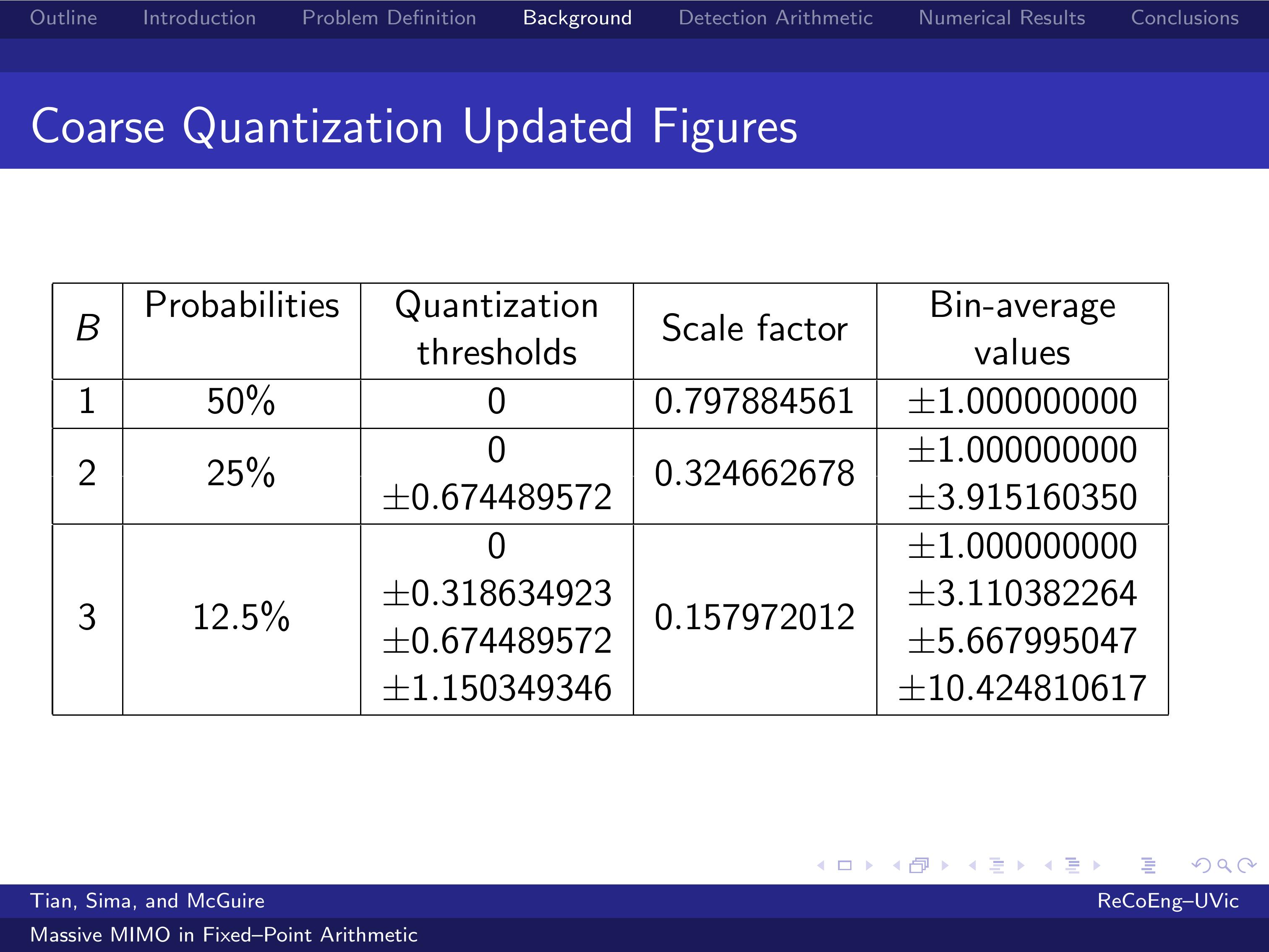 |
This table shows the updated figures.
It is apparent that the measurements of the channel output can take only a small number of different values, which is beneficial for the implementation: plus minus 1.00 in a process with one quantization bit, plus minus 1.00 and plus minus 3.91 in a process with two quantization bits, and so on.
The estimated channel coefficients, the entries of H, are also coarsely quantized to reduce the computation cost in the receiver.
I shall now review the major operations of the receiver algorithm implemented in fixed-point arithmetic with reduced precision.
|
| ICACT20210153 Slide.11
[Big Slide]
|
Chrome Click!! |
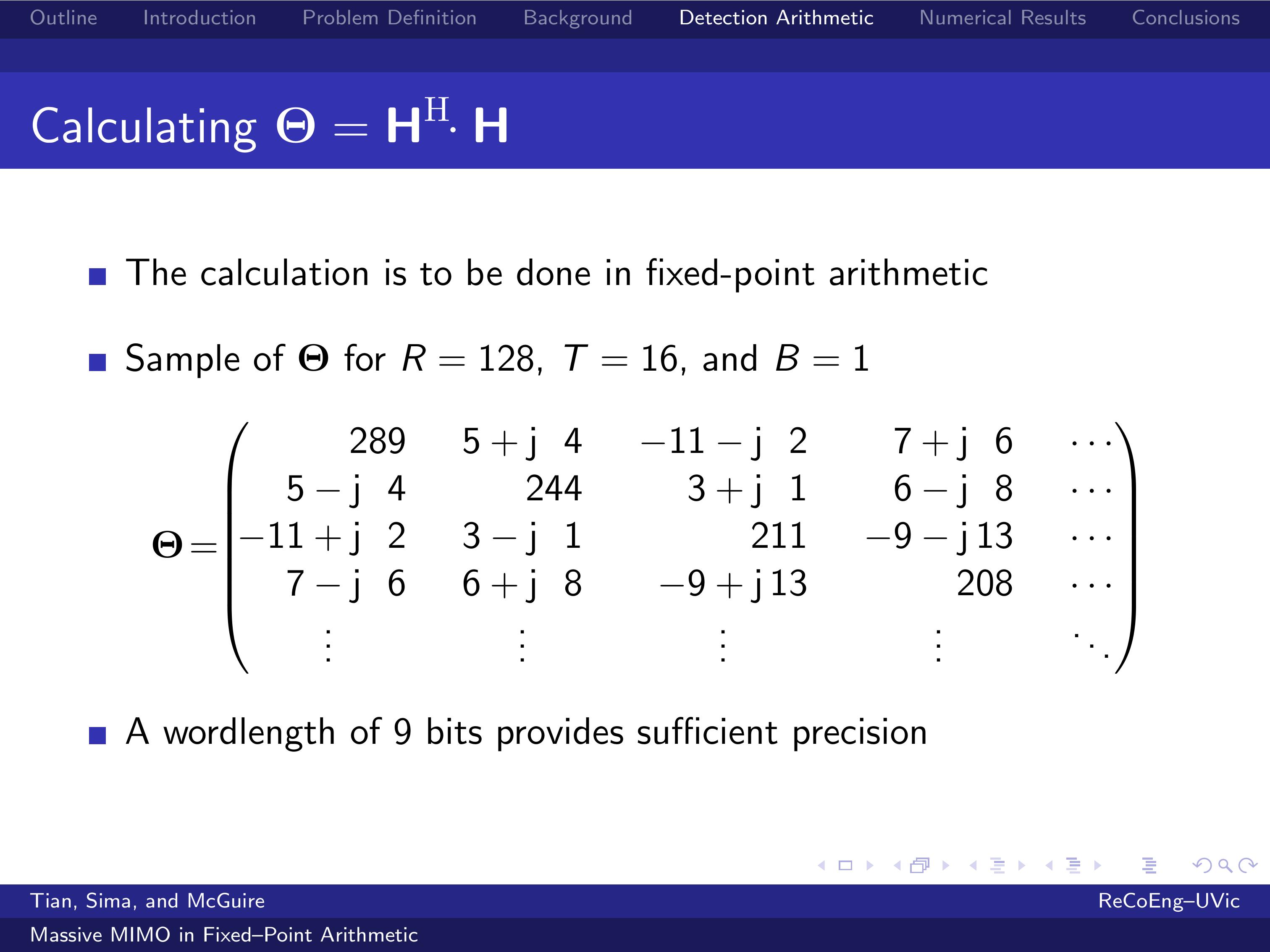 |
Due to their length and random nature, data signals of different users are likely to have very low correlation with each other.
For this reason, the Hermitian matrix Theta is diagonal dominant.
This figure shows a sample of the reduced-wordlength matrix Theta in a Massive MIMO configuration with 128 receive antennas,
16 transmit (or user) antennas, and 1 quantization bit.
Based on the statistics we collected, a wordlength of 9 bits provides sufficient precision to store each element of the matrix Theta.
Before eigenvalue decomposition, a Hessenberg decomposition is performed. However, this is not discussed here for simplicity.
|
| ICACT20210153 Slide.12
[Big Slide]
|
Chrome Click!! |
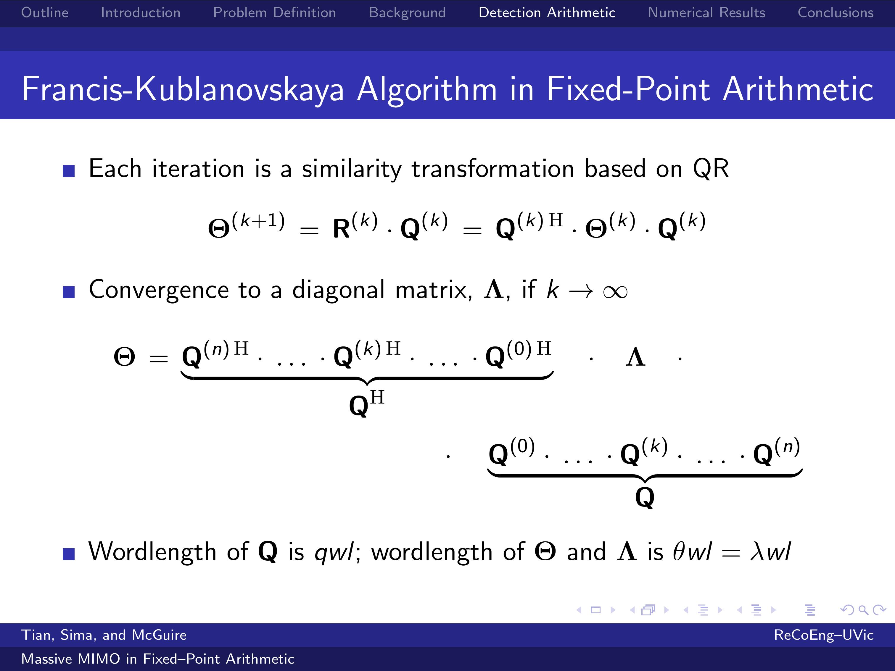 |
The Francis-Kublanovskaya recursion, in which each iteration is a similarity transformation based on the QR decomposition, is used to calculate the eigenvalue decomposition of the Hermitian matrix Theta.
At iteration k, the matrix Theta(k) is decomposed into the product of a unitary matrix Q(k) and an upper triangular matrix R(k).
By multiplying R(k) by Q(k), a similarity transformation of the matrix Theta(k) is obtained.
If k approaches infinity, then the matrix Theta(k) converges to a diagonal matrix, Lambda, whose elements are the eigenvalues of the initial Theta.
The wordlength of Q is qwl, and the wordlength of Theta and Lambda is theta wl = lambda wl.
|
| ICACT20210153 Slide.13
[Big Slide]
|
Chrome Click!! |
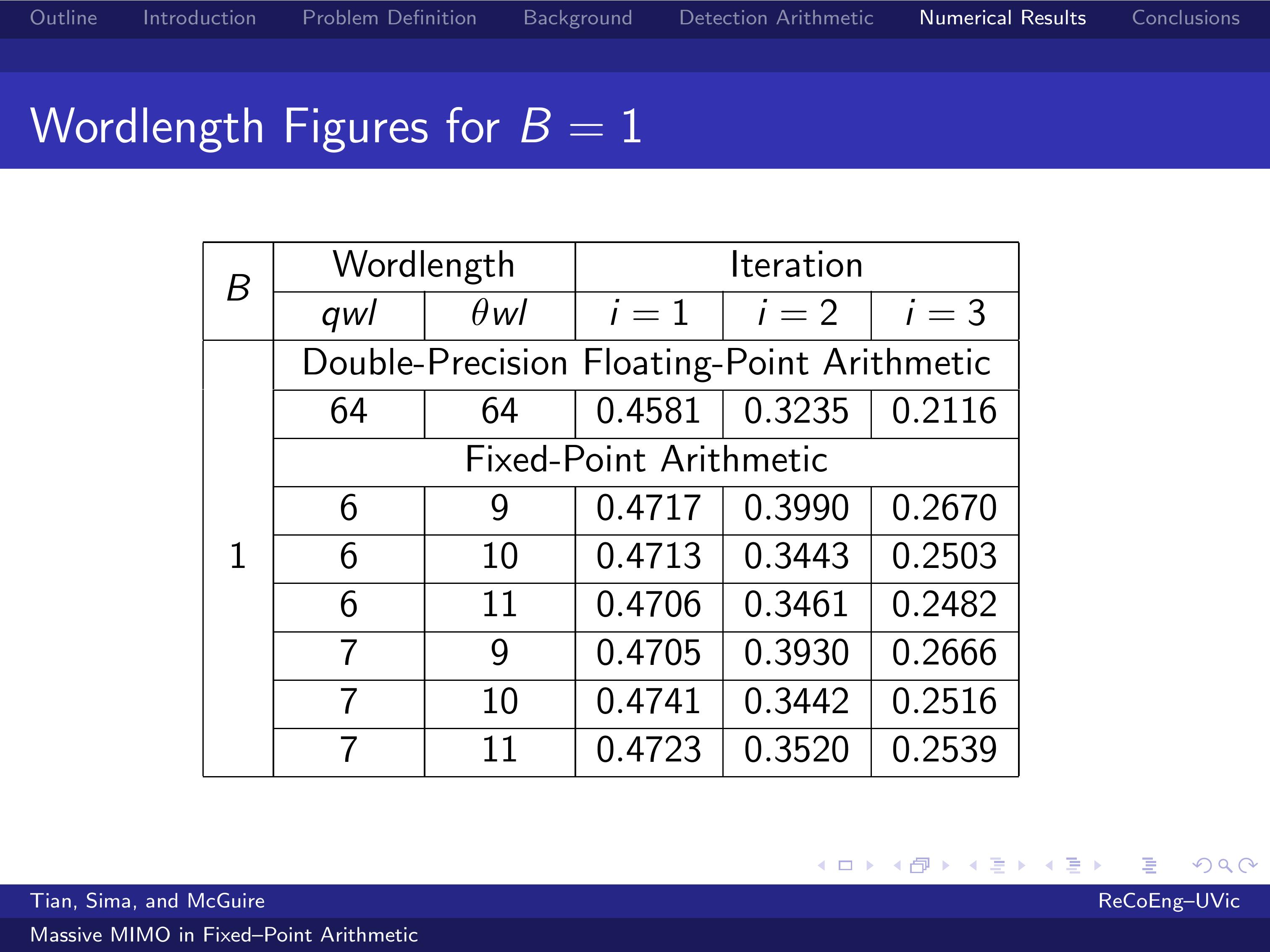 |
The challenge of designing a Massive MIMO base station is to minimize the wordlengths qwl and theta wl while the Bit-Error Rate is maintained at acceptable levels.
The iterative channel estimator used in our prior work has been converted to use only fixed-point arithmetic.
The wordlength of matrix Q was set to 6 and 7 bits.
The wordlength of matrix Theta was set to 9, 10, and $11$.
The number of quantization bits were set to 1, 2, and 3.
It is apparent that for a coarse quantization with 1 bit, neither the floating-point nor the fixed-point implementations
do not achieve a satisfactory Bit-Error Rate in a small number of iterations.
|
| ICACT20210153 Slide.14
[Big Slide]
|
Chrome Click!! |
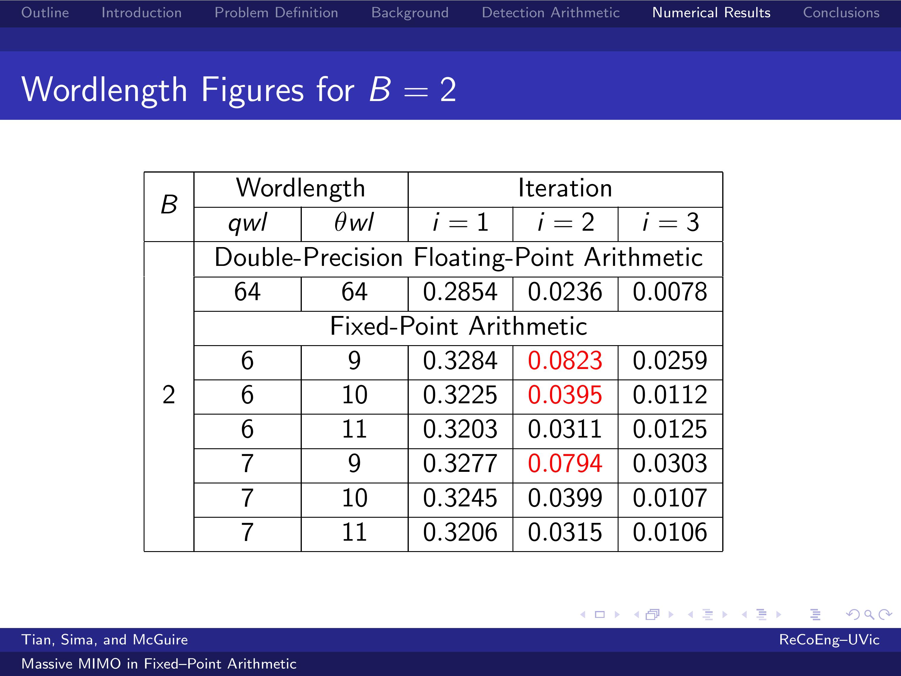 |
For a coarse quantization with 2 bits, three to four iterations generally suffices to achieve a good Bit-Error Rate.
It is observed that an additional iteration is generally needed in fixed-point implementation over the floating-point implementation to match their Bit-Error Rates.
It is also apparent that for a quantization with 2 bits, the worldength of Q has little impact on the Bit-Error Rate: 0.0823 is achieved for qwl=6, and 0.0794 is achieved for qwl=7.
On the other hand, the wordlength of Theta has a much stronger impact on the Bit-Error Rate: 0.0823 is achieved for theta wl=9, and 0.0395 is achieved for theta wl=10.
|
| ICACT20210153 Slide.15
[Big Slide]
|
Chrome Click!! |
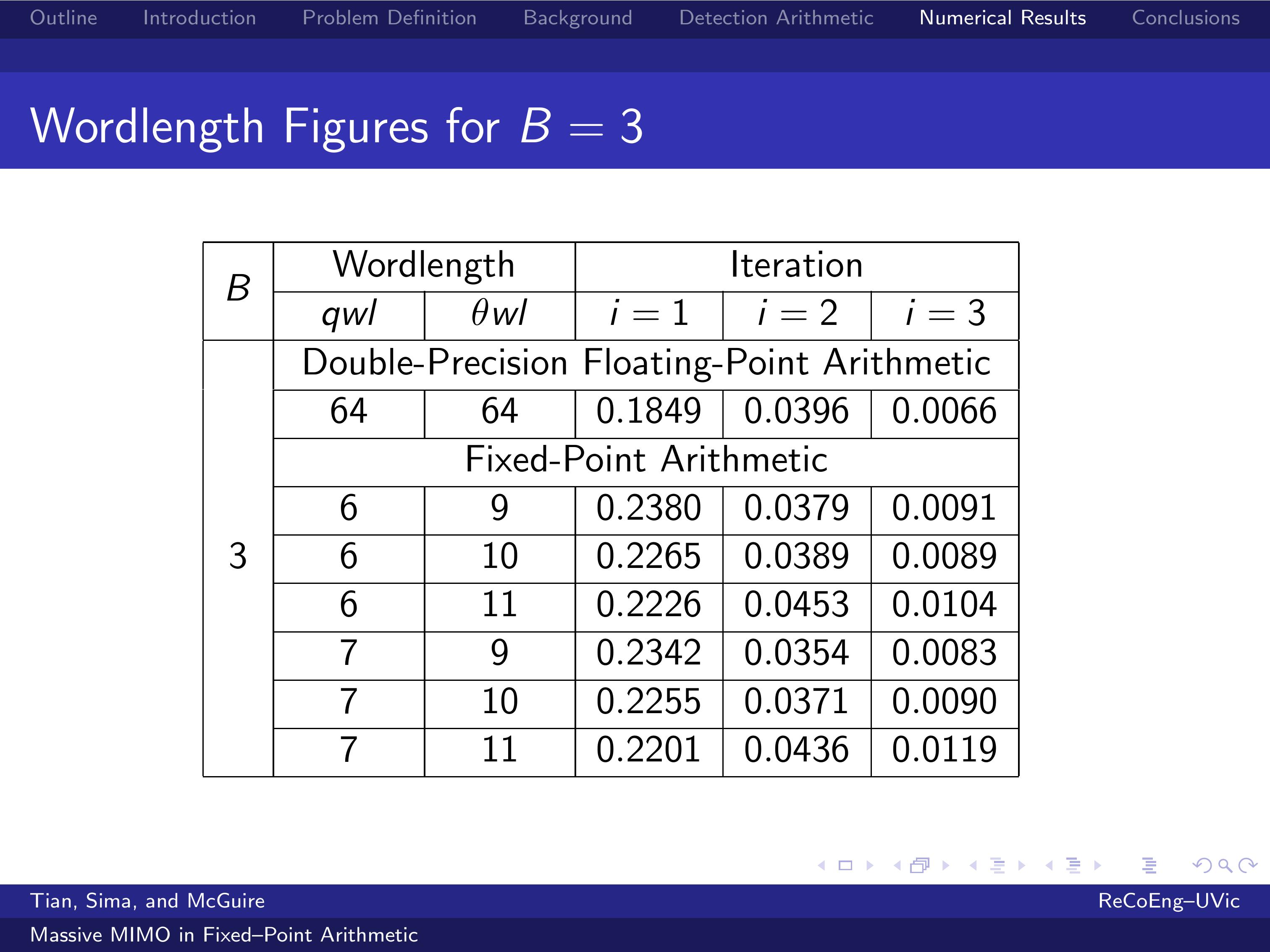 |
The results for 2 and 3 quantization bits are similar.
For a coarse quantization with 3 bits, three to four iterations generally suffices to achieve a good Bit-Error Rate.
It is observed that an additional iteration is generally needed in fixed-point implementation over the floating-point implementation to match their Bit-Error Rates.
It is apparent that a coarsely quantized MMIMO system with B=3 is robust enough and can operate with theta wl =9, but the cost of the implementation will be higher due to the increased complexity of the implementation in fixed-point arithmetic.
The Bit-Error Rate does not improve significantly for a theta wl greater than 11.
|
| ICACT20210153 Slide.16
[Big Slide]
|
Chrome Click!! |
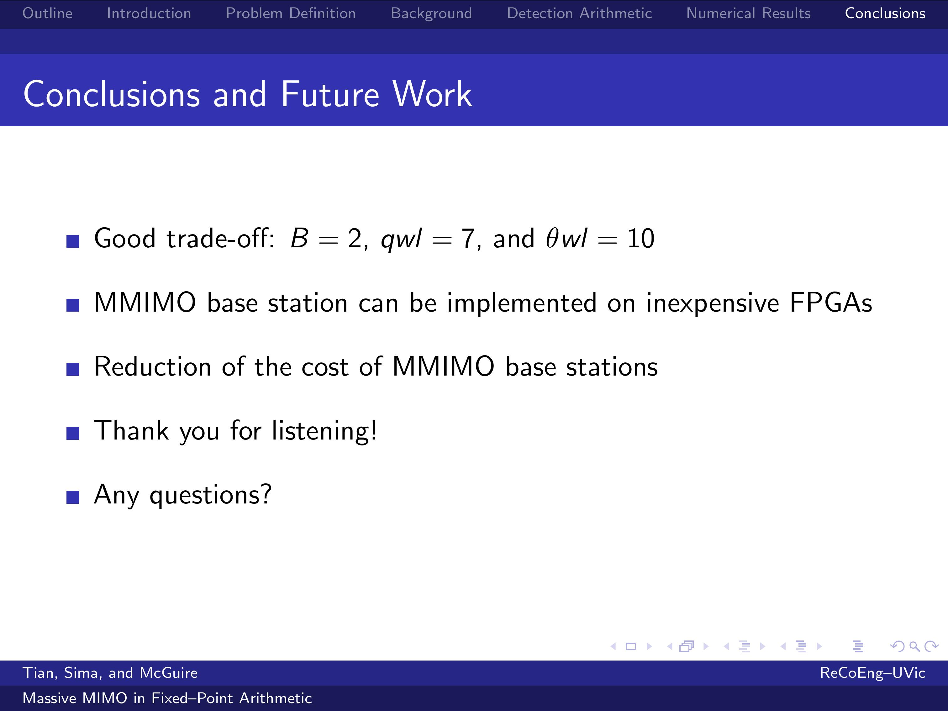 |
It is apparent that a good trade-off in implementing a Massive MIMO base station is a coarse quantization with 2 bits, a Q's wordlength of 7 bits, and a Theta's wordlength of 10 bits.
With such a reduced wordlength for matrix Q, vector rotations can be easily implemented in inexpensive hardware, such as reasonably sized Field-Programmable Gate Arrays.
This allows the reduction of the cost of massive MIMO base stations, which is a key impediment to their widespread deployment.
This last statement completes my talk.
If there are any questions, I shall be glad to take them.
Thank you for listening!
|