Now 4800 visitors
Today:0 Yesterday:0
Total: 145473
215S 51P 5R
2026-10-21, Week 43 |
| Member Login |
| TACT Journal Homepage |
| Call for Paper |
| Committee |
| Find My Paper |
| Author Homepage |
| Statistics & History |
| Welcome Message |
| Paper Procedure |
| FAQ |
| Paper Archives |
| Outstanding Papers |
| Author Homepage |
| - Paper Procedure |
| - Journal Procedure |
| - Presentation Tips |
|
| Program & Proceedings |
| Program with Papers |
| Plenary Session |
| Tutorial Session |
|
| Presentation Platform |
| Hotel & Travel Info |
| About Korea |
| Accommodation |
| Transportation |
| VISA |
| Other Infomation |
|
| Photo Gallery |
| Scheduler Login |
| Seminar |
| Archives Login |
|
| Sponsors |

|

|

|

|

|

|

|

|

|

|
|
|
|
|
 ICACT20240208 Slide.00
[Big Slide]
[YouTube] |
Chrome  Click!! |
 |
Paper No:20240208
Title: Physics-Informed Neural Networks for solving Blood Flows
Reporter: Jeu-Jiun Hu |
| ICACT20240208 Slide.01
[Big Slide]
[YouTube] |
Chrome Click!! |
 |
Physics-Informed Neural Networks for solving Blood Flows
My name is Jeu-Jiun Hu and came from Department of Computer Science and Information Engineering Taitung, Taiwan.
In my presentation today, I will address the topic of Physics-Informed Neural Networks for solving Blood Flows
|
| ICACT20240208 Slide.02
[Big Slide]
[YouTube] |
Chrome Click!! |
 |
First, we’ll be giving you an introduction Next, we’ll move on to method, results. and conclusions |
| ICACT20240208 Slide.03
[Big Slide]
[YouTube] |
Chrome Click!! |
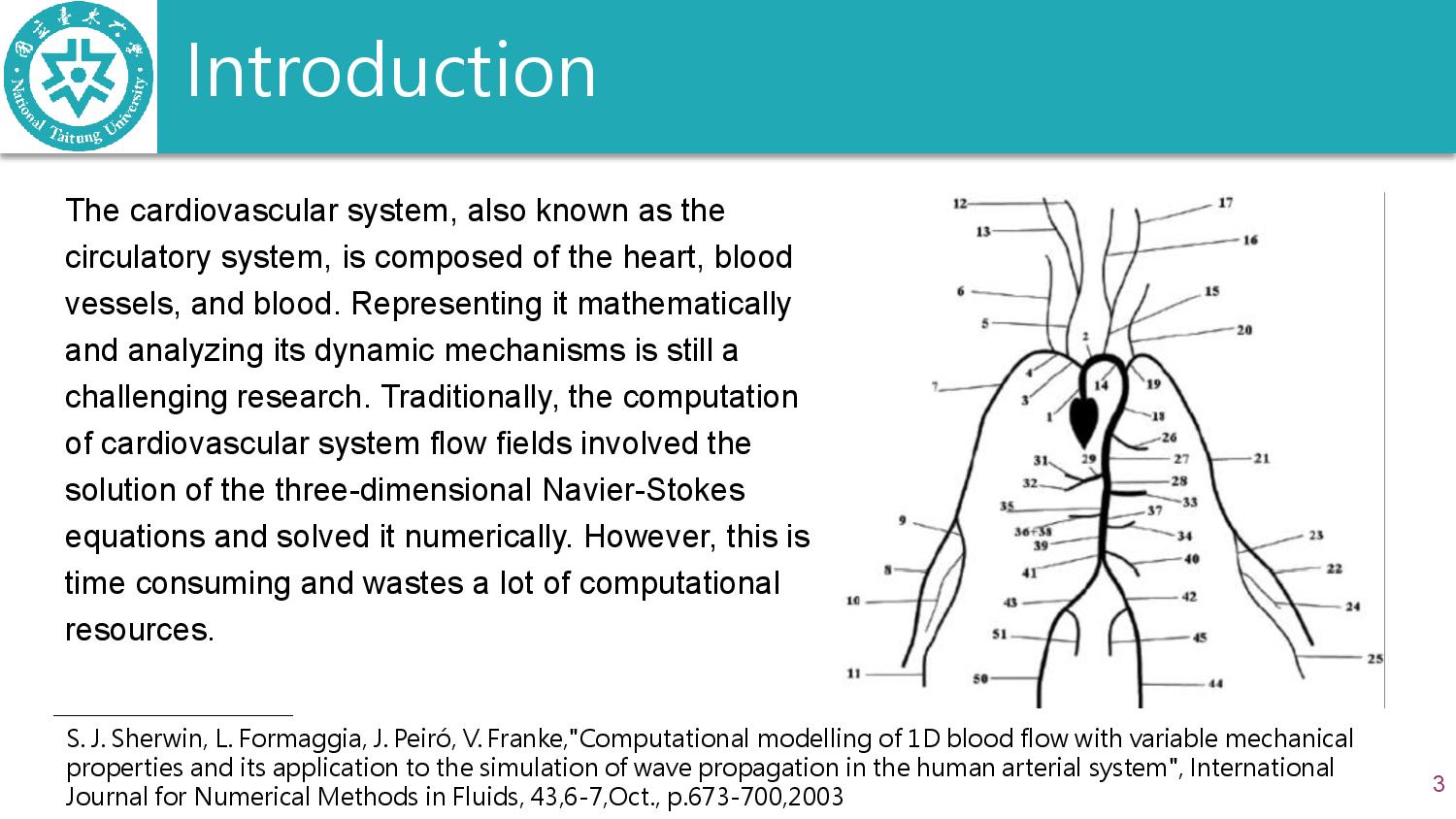 |
The cardiovascular system, also known as the circulatory system, is composed of the heart, blood vessels (arteries, veins, capillaries), and blood. Representing it mathematically and analyzing its dynamic mechanisms is still a challenging research. Traditionally, the computation of cardiovascular system flow fields involved the solution of the three-dimensional Navier-Stokes equations and solved it numerically. However, this is time consuming and wastes a lot of computational resources.
To simplify this problem, certain assumptions can be made, reducing it to a one-dimensional problem., thus, the axisymmetric Navier-Stokes equations. Axisymmetric equations may have a single point where the radius is zero making numerical solutions singularity.
In recent years, the development of Artificial Intelligence (AI) has been one of the hottest topics. Physics-informed Neural Networks (PINN), proposed by scholar M. Raissi, are a type of neural network that uses physical equations as computational constraints for solving partial differential equations. They belong to the supervised learning category. This network utilizes data-driven training, learning through loss functions described by partial differential equations. During the training process, PINN benefits from the constraints imposed by physical equations, enabling it to learn fundamental physical laws such as mass and momentum conservation. In recent years, PINN has gradually become a focal point in machine learning and computational fluid dynamics, achieving significant progress in both theory and applications.
To enhance the performance of computation of cardiovascular system flow fields, the systems can be treated as 1D tube like structures and PINN method is adopted for simulations. Further, we solve several preambles to demonstrate obtaining the results accuracy and efficiency.
|
| ICACT20240208 Slide.04
[Big Slide]
[YouTube] |
Chrome Click!! |
 |
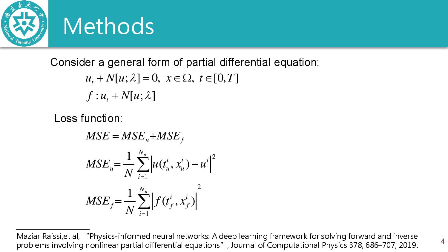
Consider a general form of partial differential equation as an example, assuming that the function u = u(t, x) and satisfies a partial differential equation in the following form:
where N[u;λ] represents a parameterized non-linear operator that operates on u with parameter λ. Ω denotes the Euclidean geometric space, and T is the terminal time. Given the initial state, boundary conditions, and physical parameter λ for u(t, x), solving the partial differential equation allows us to predict the values of u(t, x) at any spatiotemporal point. Numerical methods such as finite differences or finite elements can be employed for solving. First, let's define:
Subsequently, a neural network can be constructed to approximate the solution to the partial differential equation. Therefore, the root mean square loss function is defined as following:
the data-driven of the loss function, acquired through the initial and boundary condition in the training data, represents the physics model-driven portion of the loss function, which is trained in the system's machine learning process to approximate the neural network function. The network must not only minimize the error with known training data but also satisfy the constraints of the partial differential equation as much as possible. Therefore, the network structure and loss function of PINN need to be customized according to the form of the partial differential equation, while also maintaining the model's scalability.
PINNs - Neural networks that are trained to solve supervised learning tasks while respecting physical laws. Many physical systems consist of prior knowledge encoded in physical laws, e.g. Newton’s laws of motion. This prior information can act as a regularization constraint that reduces the space of admissible solutions , remove unrealistic solutions that violate fundamental conservation laws mass, momentum, energy
|
| ICACT20240208 Slide.05
[Big Slide]
[YouTube] |
Chrome Click!! |
 |
The Loss function |
| ICACT20240208 Slide.06
[Big Slide]
[YouTube] |
Chrome Click!! |
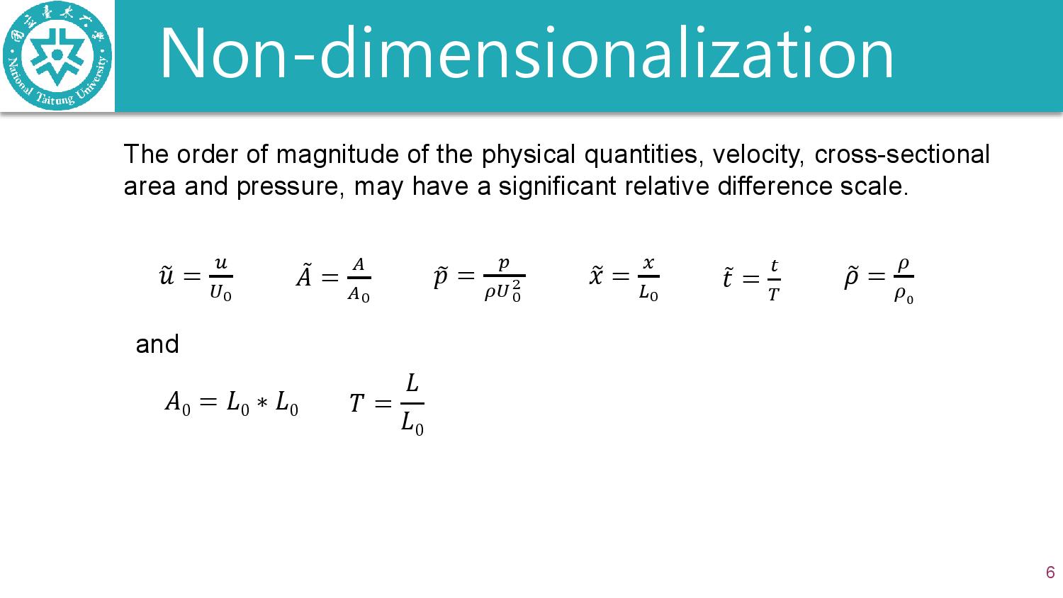 |
The order of magnitude of the physical quantities, velocity, cross-sectional area and pressure, may have a significant relative difference scale.
|
| ICACT20240208 Slide.07
[Big Slide]
[YouTube] |
Chrome Click!! |
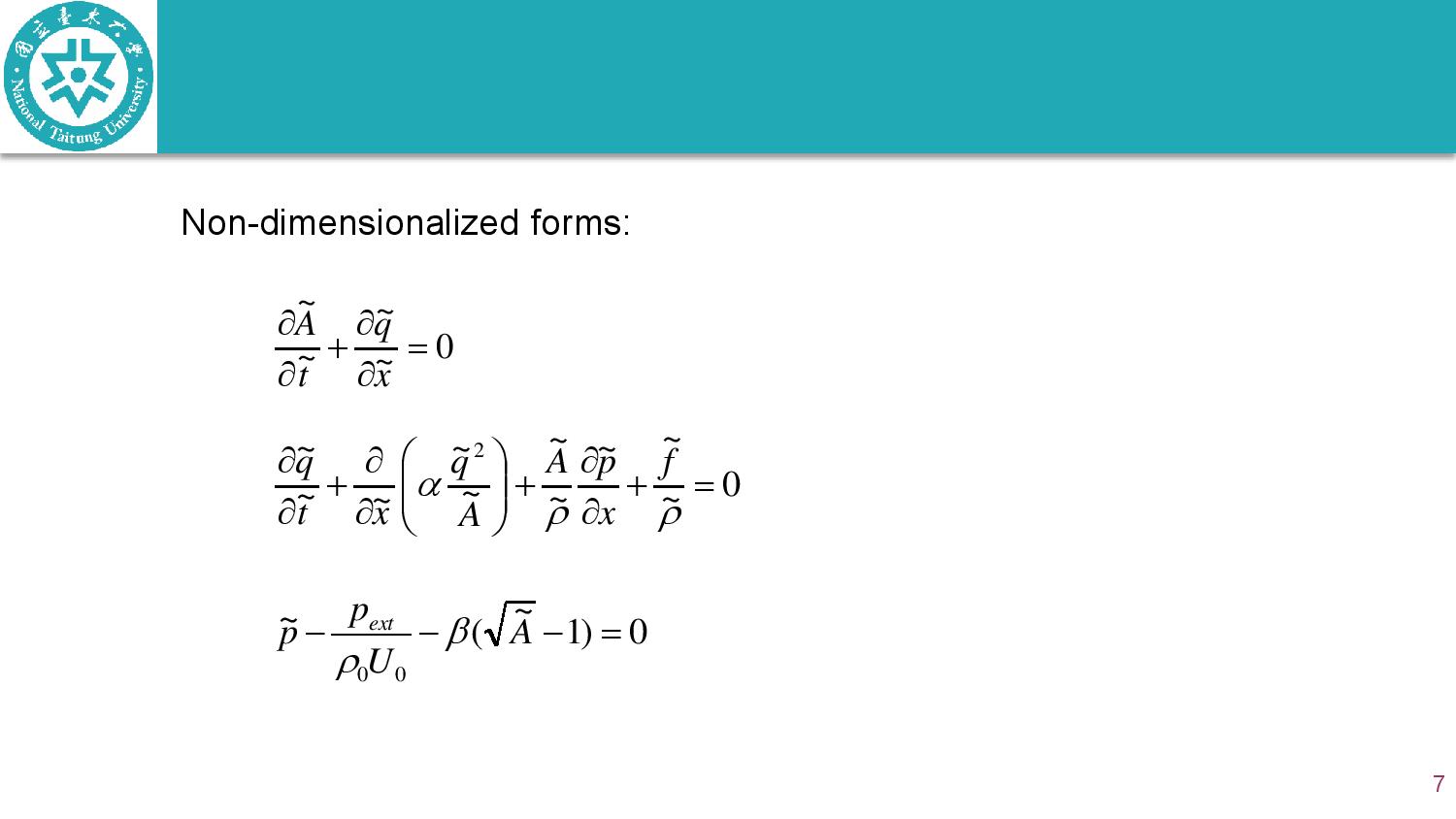 |
This is the non-dimensionalized and normalized form of the governing equations that is employed as a physical constraint in the residual part of the loss function.
|
| ICACT20240208 Slide.08
[Big Slide]
[YouTube] |
Chrome Click!! |
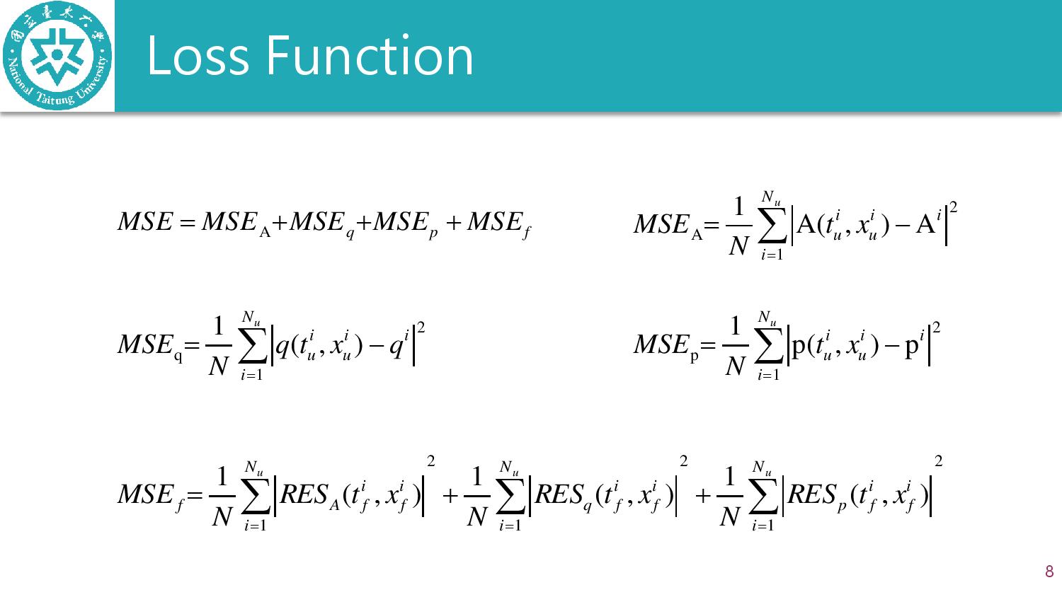 |
we provided details on how to construct the individual terms of the loss function corresponding to the measurements, physical constraints and continuity, that the model should satisfy. In this section, we will show how to combine these individual terms to create the joint form of the loss function, together with some examples to clarify the procedure. The loss function of our physics informed neural networks (PINNs) takes the form:
This complete form of the loss function that encourages the model to learn the underlining physics of the problem by using measurements inside the domain, not necessarily at the boundaries and by respecting the imposed physical constraints.
|
| ICACT20240208 Slide.09
[Big Slide]
[YouTube] |
Chrome Click!! |
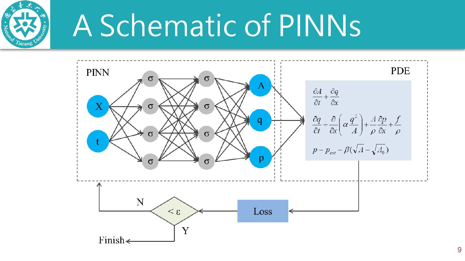 |
The loss function that corresponds to the residual losses as shown In figure, the left part represents the part of the loss function that corresponds to the interface losses and the red colored box represents the measurement loss. The different parts construct the complete loss function, by minimizing which the neural network parameters are tuned.
|
| ICACT20240208 Slide.10
[Big Slide]
[YouTube] |
Chrome Click!! |
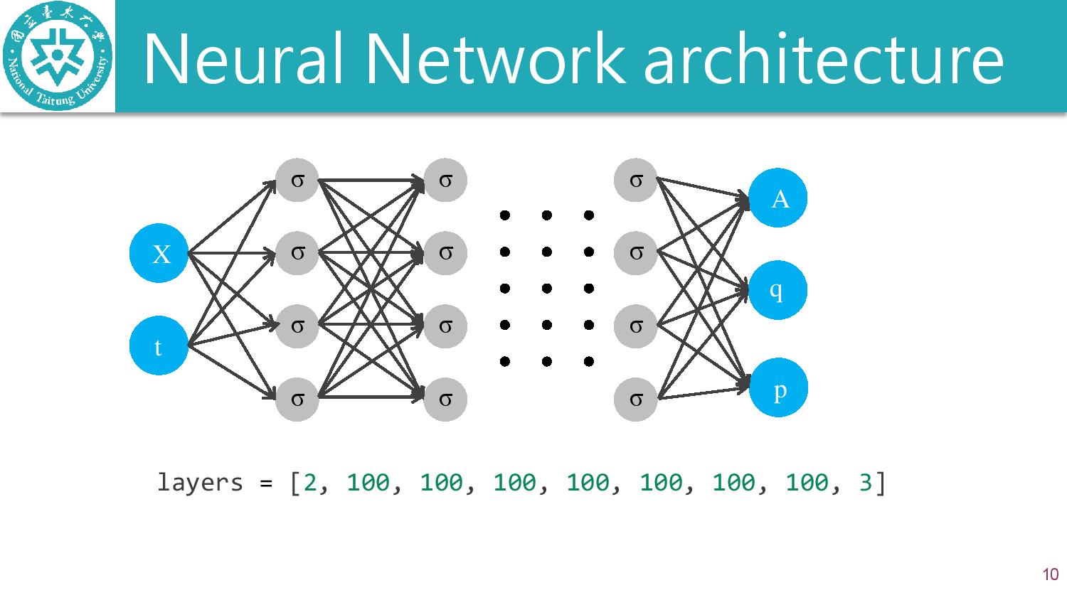 |
The problem is addressed by utilizing neural networks with seven hidden layers, each consisting of 100 neurons, and employing a hyperbolic tangent activation function.
This architecture has enough capacity to efficiently capture fine features in the propagating waveforms.
The neural networks take the scaled inputs [ ˆx, tˆ] and predict the non-dimensional outputs [A, u, p]
We are providing each neural network with velocity and cross-sectional area time series for one point at the inlet and the two outlets of the arterial network.
Using this data we infer the solution of 2, 000, randomly chosen collocation points, inside each domain, and = 1024 interface points. Moreover we choose batches of 1, 024 points as input and learning rate η = 10−3 for the first 90, 000 iterations. Consequently, we set η = 10−4 for the following 40, 000 for further minimizing the error and fine-tuning the neural network parameters.
|
| ICACT20240208 Slide.11
[Big Slide]
[YouTube] |
Chrome Click!! |
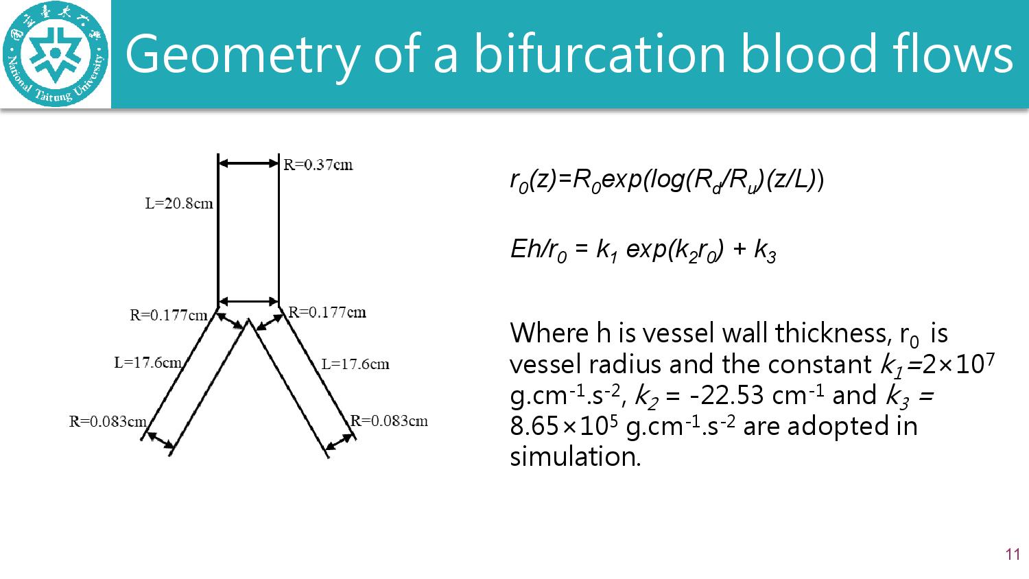 |
Geometry of a bifurcation blood flows.
|
| ICACT20240208 Slide.12
[Big Slide]
[YouTube] |
Chrome Click!! |
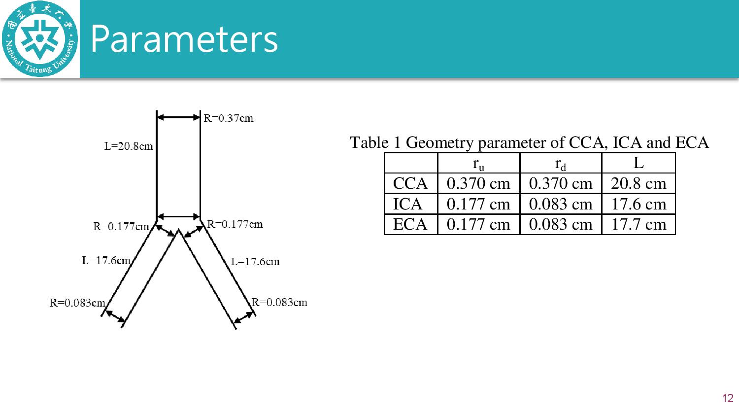 |
Geometry parameter of CCA, ICA and ECA |
| ICACT20240208 Slide.13
[Big Slide]
[YouTube] |
Chrome Click!! |
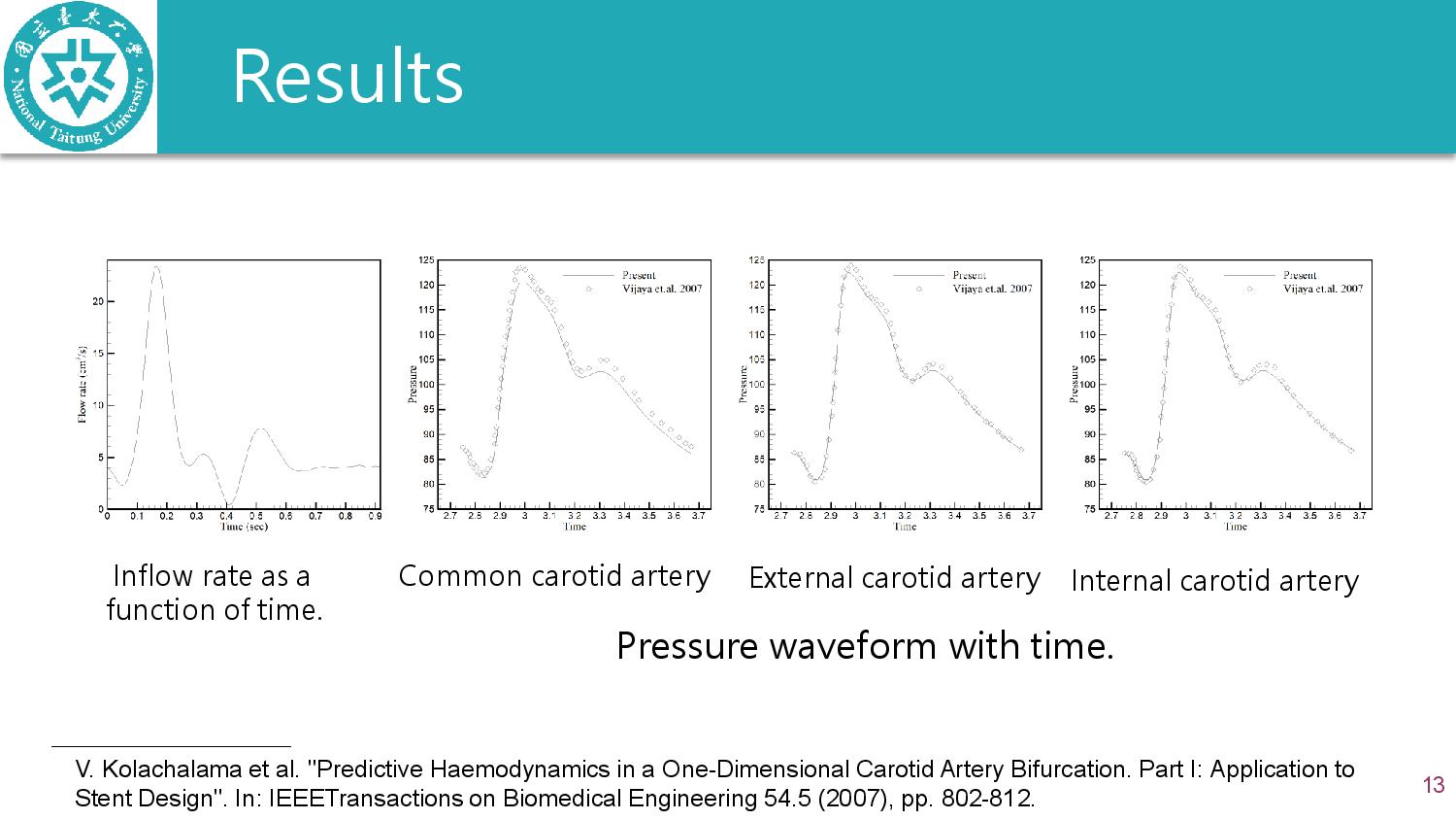 |
We assume we have obtained data for cross-sectional area and velocity at the inlets and outlets of a prototype carotid bifurcation. Our goal is given these measurements, to predict the values of the pressure at the middle points of the domain. We present the results for the case of non-dimensionalized physics informed neural networks and the reference solution acquired by other paper.
The pressure waveform at various locations in a bifurcation vessel, obtained through the application of the PINN method to solve the 1-D equations, is illustrated in Figure.
Specifically, the plots are at a location 6 cm from the common carotid artery, internal carotid artery, and external carotid artery.
The results compared well with other papers.
|
| ICACT20240208 Slide.14
[Big Slide]
[YouTube] |
Chrome Click!! |
 |
The PINN method is employed to simulate one-dimensional blood flows.
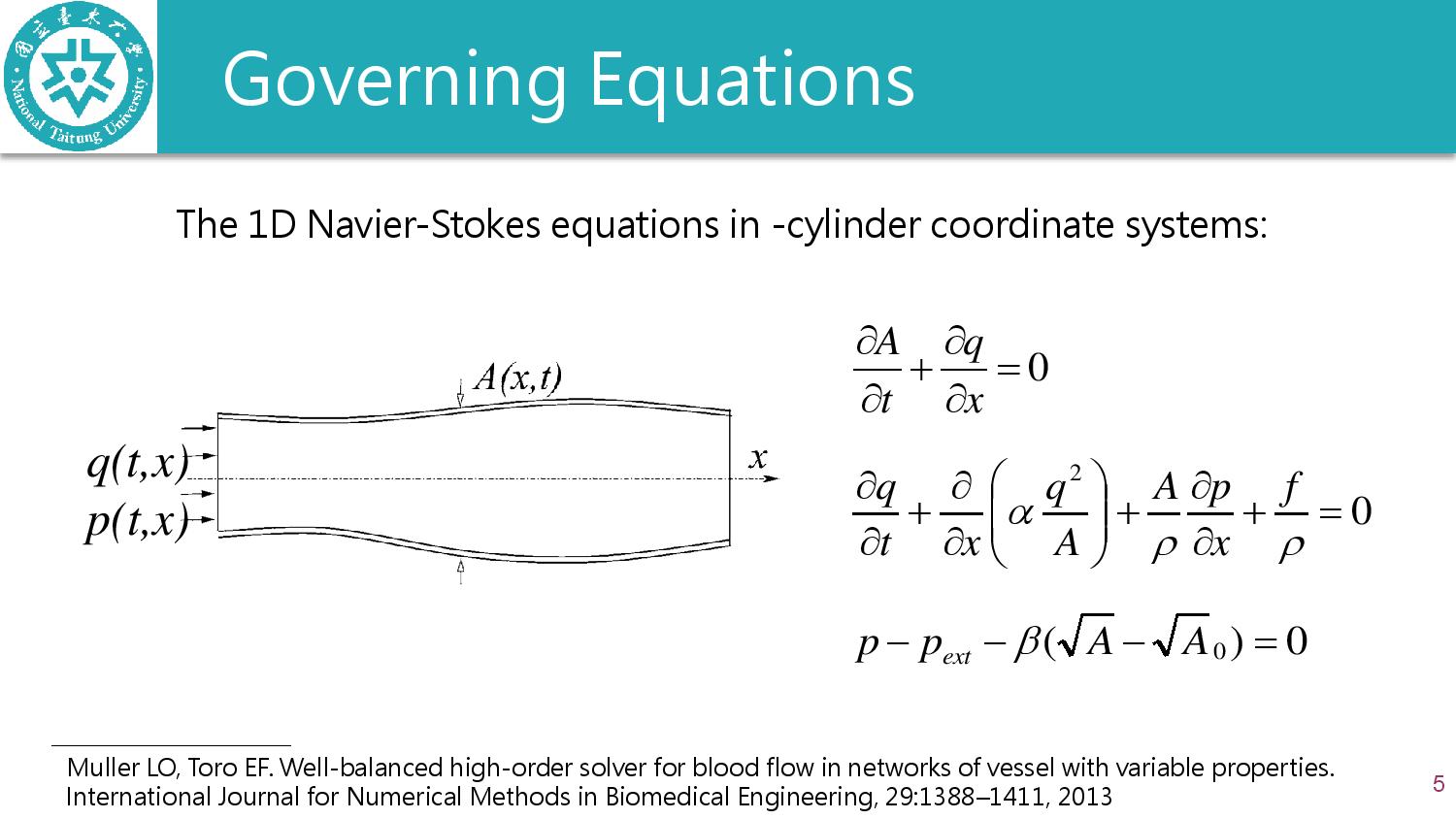
One-dimensional Navier-Stokes equations in cylindrical coordinate systems.
The proposed PINN method's results are compared well with others papers.
The results demonstrate that the PINN method functions as expected
Demonstrations indicate that considering bifurcation pressure drops can significantly enhance accuracy.
Consequently, achieving comparable accuracy in blood flow solutions for 1D models using the PINN method compared to traditional numerical methods for 2D or 3D models is feasible.
|
| ICACT20240208 Slide.15
[Big Slide]
[YouTube] |
Chrome Click!! |
 |
Thanks |
| |