ICACT20260241 Slide.01
[Big Slide]
[YouTube] |
Chrome  Click!! |
 |
Hello, everyone. Thank you for joining today’s presentation. Our work is titled A Comparative Analysis of Machine Learning Algorithms for Intelligent Spectrum Sensing in Cognitive Radio Networks. This research is presented by myself, Md. Tofail Ahmed, along with my co-authors Mousumi Haque, Yosuke Sugiura, and Tetsuya Shimamura.
|
| ICACT20260241 Slide.02
[Big Slide]
|
Chrome Click!! |
 |
To guide our discussion, here is our outline. We will begin with an introduction to cognitive radio and the motivation for our work. Then, we will discuss both conventional and modern machine learning-based spectrum sensing methods. I will walk you through our model implementation, share the key simulation results, and finally, present our conclusion.
|
| ICACT20260241 Slide.03
[Big Slide]
|
Chrome Click!! |
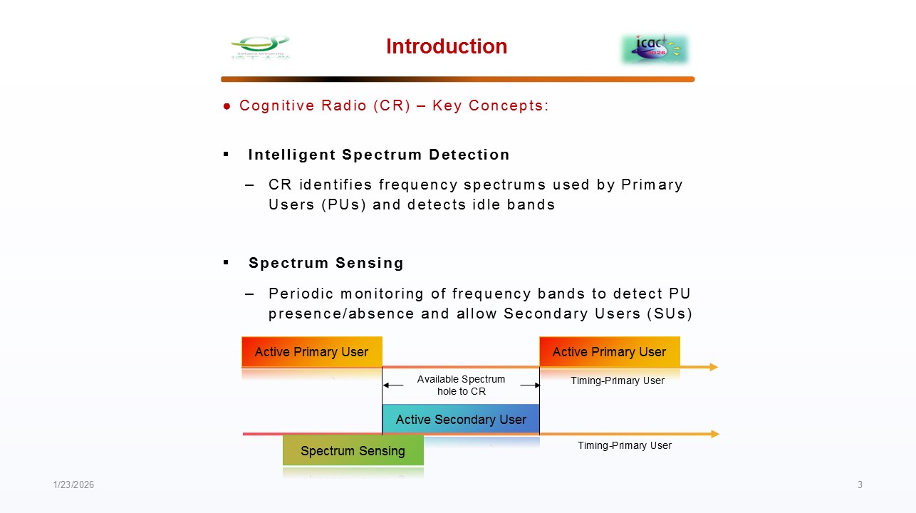 |
Lets start with the fundamentals. Cognitive radio is an intelligent wireless communication system. Its core function is spectrum sensing. It constantly monitors the radio environment to identify which frequency bands are occupied by licensed primary users (PUs) and, more importantly, to detect idle spectrum holes. These holes can then be safely used by unlicensed secondary users (SUs), improving overall efficiency.
|
| ICACT20260241 Slide.04
[Big Slide]
|
Chrome Click!! |
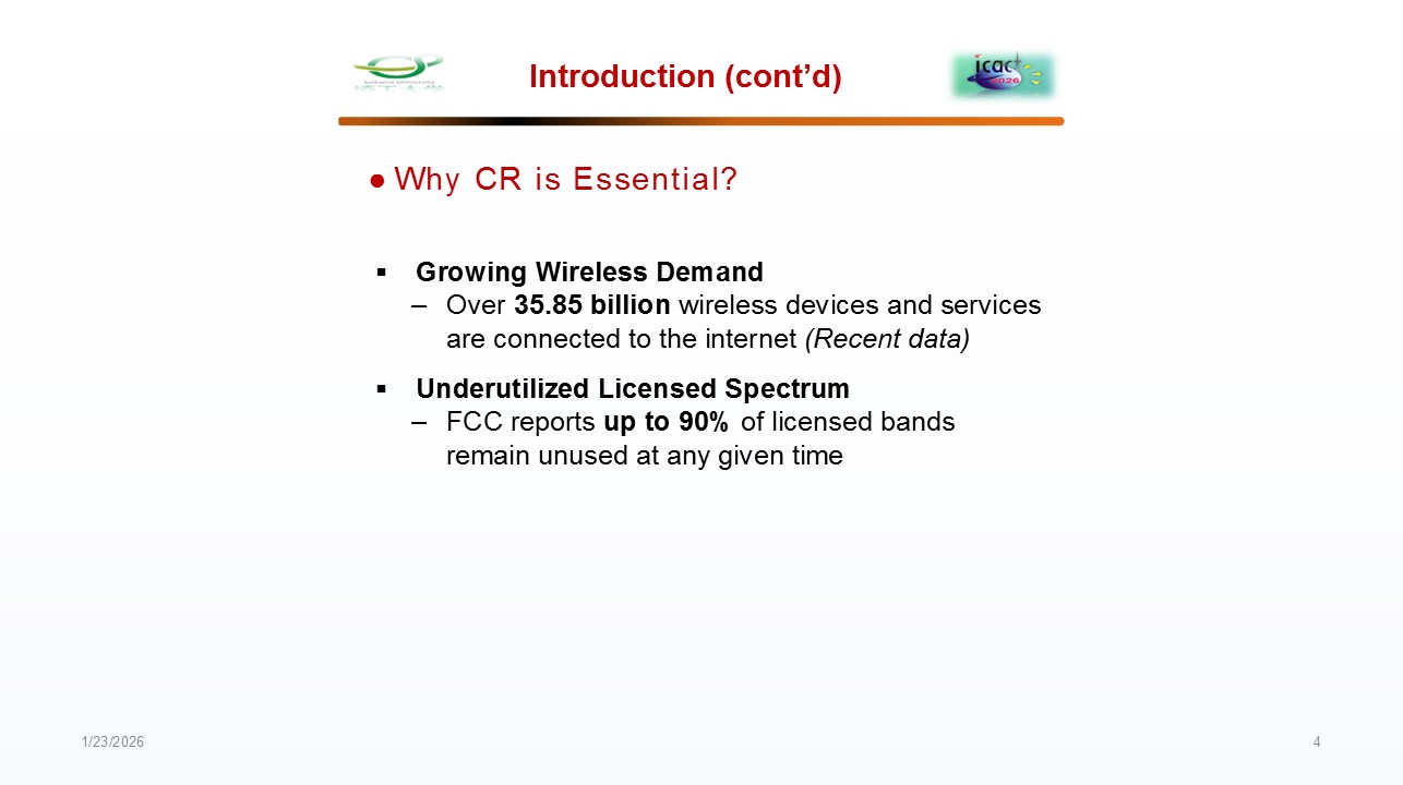 |
Why is this so critical? There are two primary reasons for this critical situation. First, the demand is exploding; recent data shows over 35.85 billion wireless devices are connected. Second, regulatory bodies like the federal communications commission (FCC) report that up to 90% of the licensed spectrum remains unused at any given time. Cognitive radio is the key technology to bridge this gap between scarcity and underutilization.
|
| ICACT20260241 Slide.05
[Big Slide]
|
Chrome Click!! |
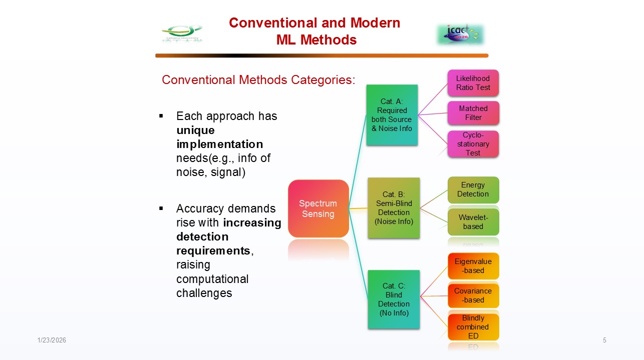 |
How do we perform this spectrum sensing? Traditionally, we have popular conventional methods like energy detection and matched filter detection. However, each method has specific requirements and faces challenges, especially as we demand higher accuracy in difficult conditions, which increases computational complexity.
|
| ICACT20260241 Slide.06
[Big Slide]
|
Chrome Click!! |
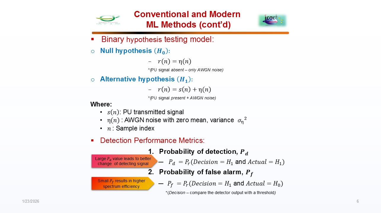 |
Let’s dive into the core statistical model behind spectrum sensing. We frame this as a binary hypothesis testing problem: H0 means only noise is present; H1 means signal plus noise. We evaluate detectors using two key metrics: probability of detection (Pd), which should be high. Pd is the probability that the detector correctly identifies the presence of the PU when it is truly there, and the probability of false alarm (Pf), which should be low. Pf is the probability that the detector incorrectly identifies the presence of the PU when it is not there. In a conventional system, every method is decided by comparing a test statistic to a threshold.
|
| ICACT20260241 Slide.07
[Big Slide]
|
Chrome Click!! |
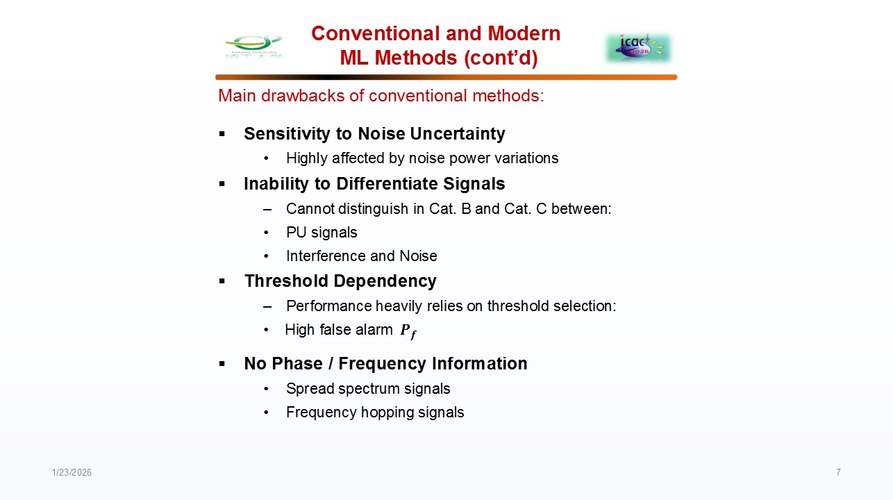 |
Why do we need machine learning in spectrum sensing? Conventional methods like energy detection come with serious drawbacks. The conventional methods are noise-sensitive, can not classify signals, depend too much on thresholds, and ignore key signal features, which makes them unreliable for modern spectrum sensing. Machine learning overcomes these limitations. |
| ICACT20260241 Slide.08
[Big Slide]
|
Chrome Click!! |
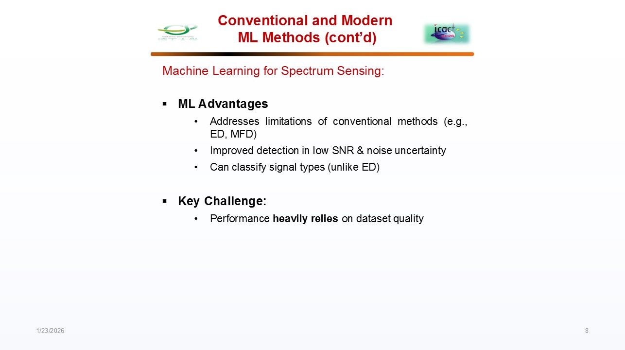 |
Diving deeper into conventional methods, while useful, has limitations in low signal-to-noise ratio (SNR) environments and under noise uncertainty. In such an environment, machine learning excels. Machine learning models can learn complex patterns, operate better in low SNR, and even classify the type of signal present. However, a major challenge remains: their performance is heavily dependent on the quality of the dataset.
|
| ICACT20260241 Slide.09
[Big Slide]
|
Chrome Click!! |
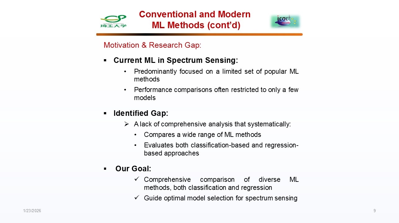 |
Let’s discuss the motivation behind this research. Currently, most research in ML-based spectrum sensing focuses on a limited set of popular algorithms. We identified a gap: a lack of a comprehensive, systematic comparison across a wide range of models, including both classification and regression approaches. Therefore, our goal is to conduct this broad analysis to provide clear guidance for optimal model selection.
|
| ICACT20260241 Slide.10
[Big Slide]
|
Chrome Click!! |
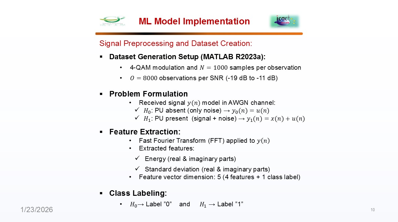 |
We built our dataset in MATLAB using 4-QAM signals in AWGN noise, from -19 to -11 dB SNR. Each observation is transformed with FFT, and we extract energy and standard deviation features from the real and imaginary parts. This provides us a 5-dimensional feature vector, labeled 0 for noise-only and 1 for signal present, which is ready for machine learning training and testing.
|
| ICACT20260241 Slide.11
[Big Slide]
|
Chrome Click!! |
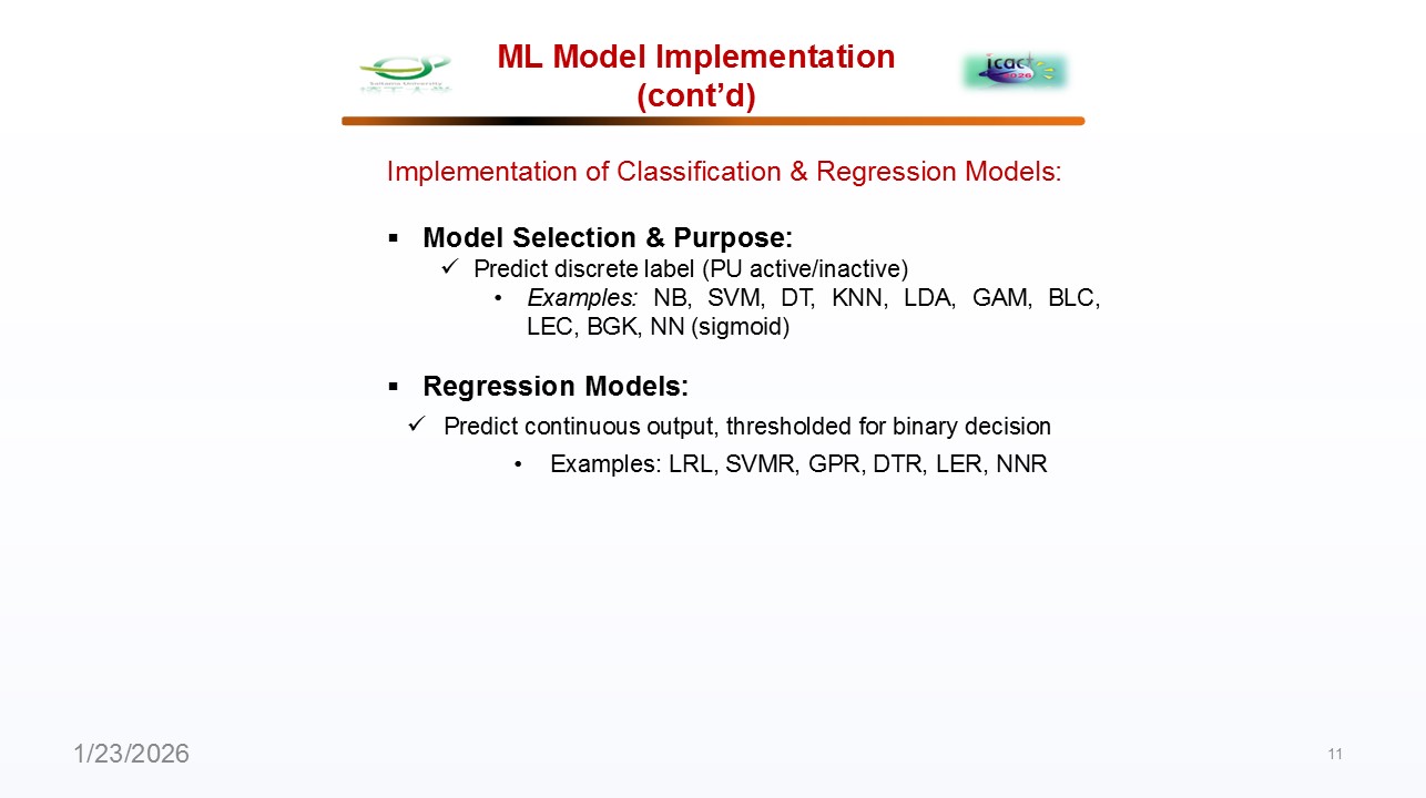 |
We test two main approaches. The first is classification models, like SVM, DT, and NN, which directly predict whether a PU signal is present or absent. The second is regression models, like SVM regression, Gaussian process regression, and LR, which output a continuous value that we then convert into a decision using a simple threshold. This setup allows us to evaluate which strategy works best for spectrum sensing in different scenarios.
|
| ICACT20260241 Slide.12
[Big Slide]
|
Chrome Click!! |
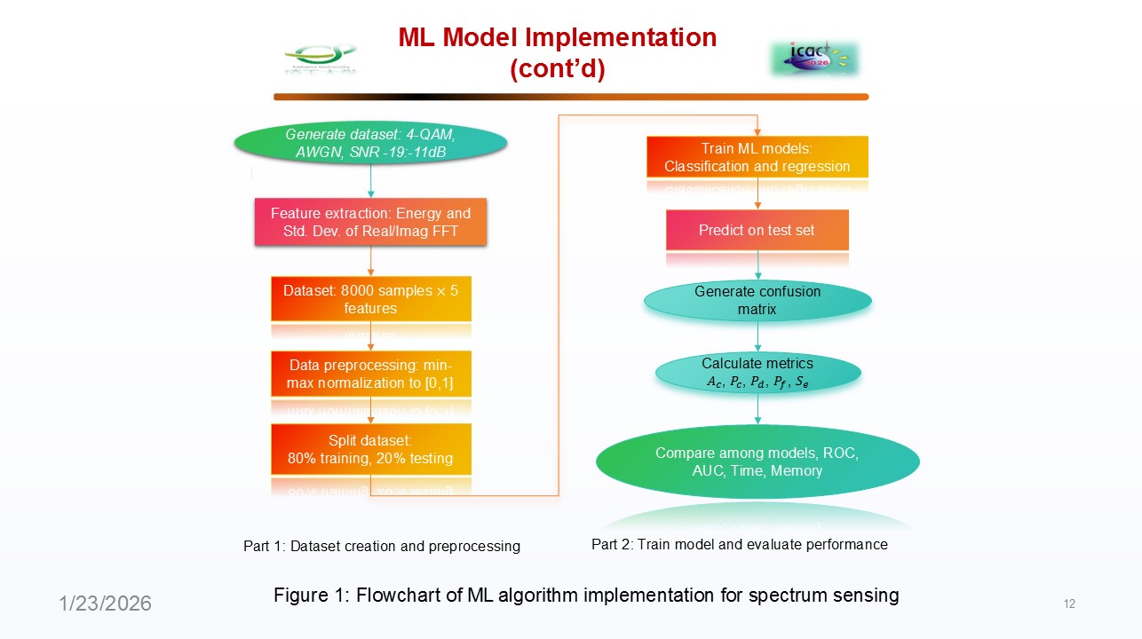 |
This flowchart illustrates our end-to-end machine learning pipeline for intelligent spectrum sensing. We begin with dataset generation and preprocessing, where we simulate signals, extract features, and prepare the training data. Next, we move to model training, where multiple classification and regression algorithms are trained simultaneously for a comprehensive comparison. Once trained, each model enters the evaluation phase, where we measure key performance metrics, like detection probability and false alarm rate, against the test dataset. Finally, based on this evaluation, the system makes a sensing decision, selecting the best-performing model to deploy for real-time spectrum detection.
|
| ICACT20260241 Slide.13
[Big Slide]
|
Chrome Click!! |
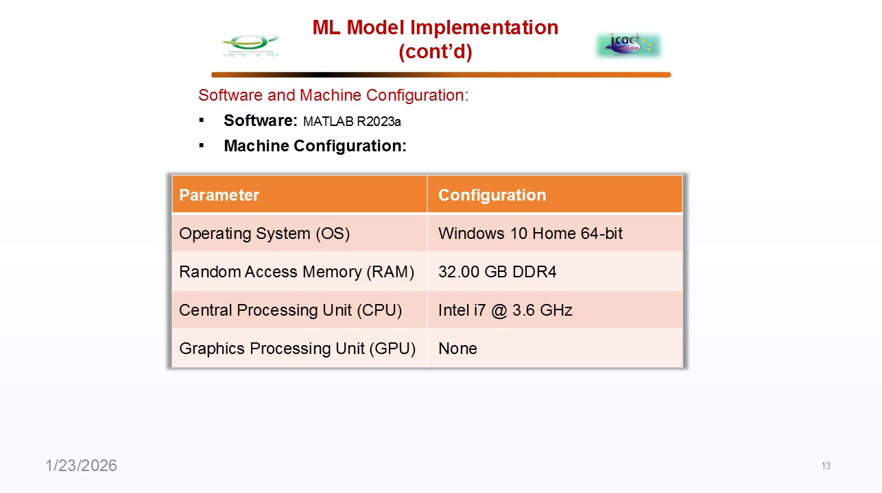 |
All of our work was done in MATLAB 2023a on a Windows 10 computer with 32GB of RAM and an Intel i7 processor. A key point is that we did not use a graphics processing unit (GPU); all results came from the CPU alone, so our performance data reflects pure processing speed.
|
| ICACT20260241 Slide.14
[Big Slide]
|
Chrome Click!! |
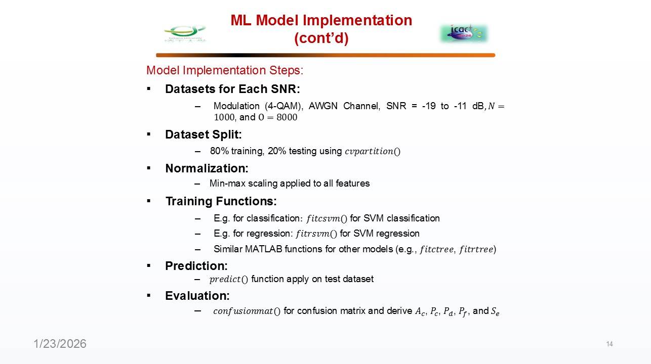 |
Now, let me walk you through the exact steps of how we implement and train our machine learning models. Our dataset is simulated with input signals (4-QAM, AWGN channel) across low SNR values from -19 to -11 dB. We split the data 80/20 for training/testing, normalize the features, and train models using MATLAB functions like the fitcsvm() function for classification and the fitrsvm() function for regression. Predictions are made with the predict() function, and performance is evaluated using metrics derived from the confusionmat() function, including accuracy, precision, Pd, Pf, and sensing error. |
| ICACT20260241 Slide.15
[Big Slide]
|
Chrome Click!! |
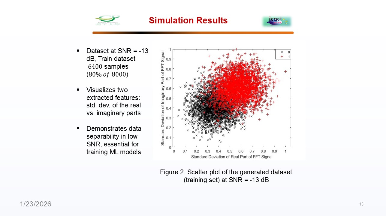 |
Lets look at the results. First, this scatter plot shows a snapshot of our training data at a very challenging SNR of -13 dB. You can see the distribution and overlap between the signal present and noise only classes, which sets the challenges for different classification models to accurately identify the PU.
|
| ICACT20260241 Slide.16
[Big Slide]
|
Chrome Click!! |
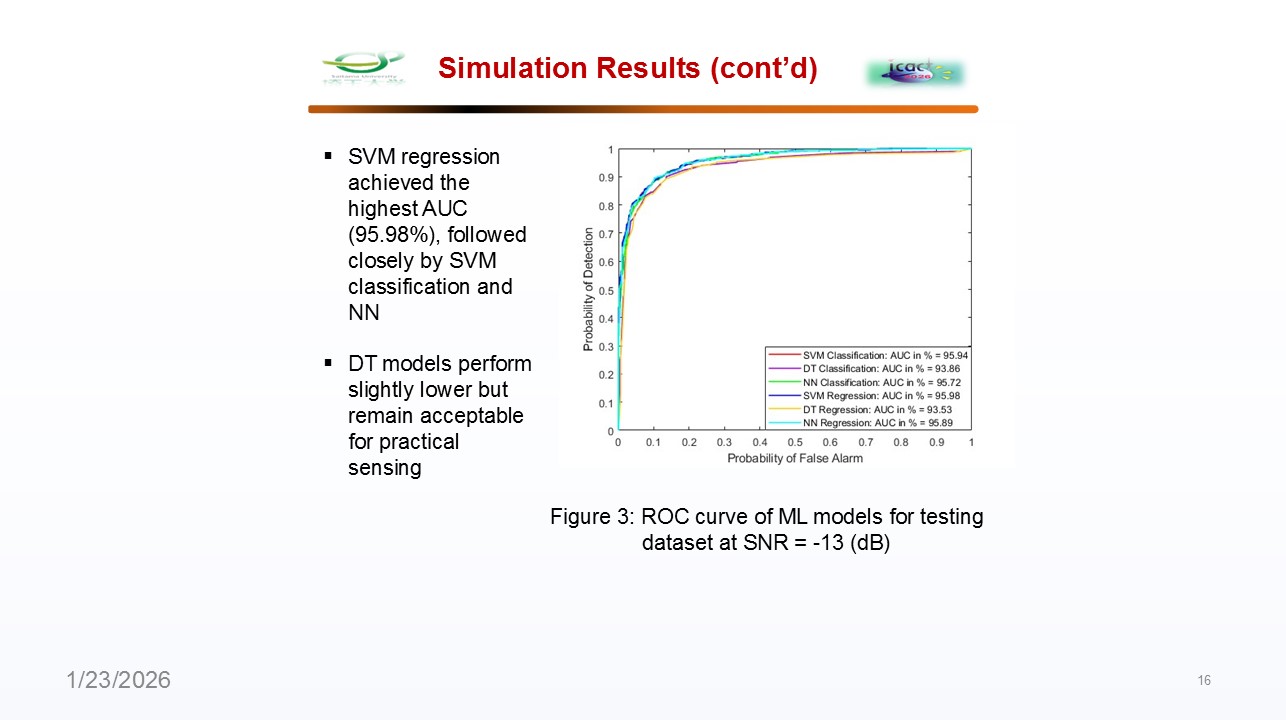 |
The performance is best summarized by the receiver operating characteristic (ROC) curves at that same low SNR. As you can see, SVM regression achieves the highest area under the curve (AUC) at 95.98%, closely followed by SVM classification and neural networks. Decision tree models, while slightly lower, still perform at an acceptable level for practical use.
|
| ICACT20260241 Slide.17
[Big Slide]
|
Chrome Click!! |
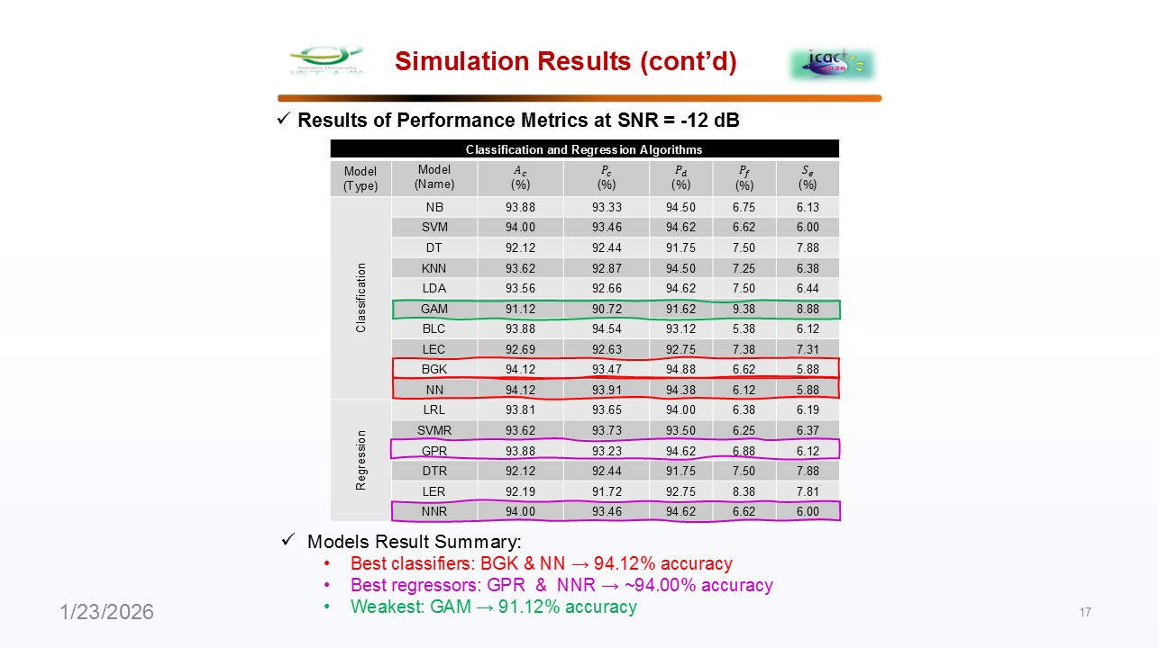 |
At a slightly higher SNR of -12 dB, we see the accuracy metrics. The top performers in this test are the binary Gaussian kernel (BGK) with logistic learner classifiers and neural networks for classification, as well as Gaussian process regression (GPR) and neural network regression for regression tasks, all of which achieve around 94% accuracy. The generalized additive model, or GAM, is the weakest in this test.
|
| ICACT20260241 Slide.18
[Big Slide]
|
Chrome Click!! |
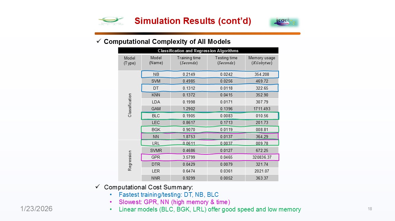 |
But accuracy is not everything; we must consider computational cost. The simplest models, like decision trees and naïve Bayes, are the fastest to train and test. The most complex models, like Gaussian process regression and neural networks, offer high accuracy but at a significant cost in memory and processing time. Linear models provided an excellent balance of adequate speed and reasonable performance. |
| ICACT20260241 Slide.19
[Big Slide]
|
Chrome Click!! |
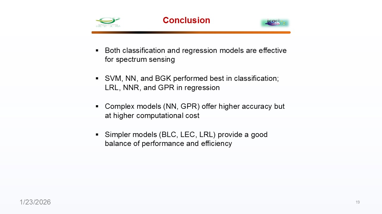 |
In conclusion, our comprehensive analysis shows that both classification and regression models are highly effective for spectrum sensing. For top accuracy, consider SVM, neural networks, or BGK classifiers. If you need a balance of performance and efficiency, simpler linear models are a strong choice. The best model ultimately depends on your specific system constraints, such as whether you prioritize absolute detection accuracy or computational resources.
|
| ICACT20260241 Slide.20
[Big Slide]
|
Chrome Click!! |
 |
That concludes our presentation. Thank you for your attention. We are now happy to take any questions you may have. |