Now 5046 visitors
Today:0 Yesterday:0
Total: 147043
212S 50P 4R
2026-10-20, Week 43 |
| Member Login |
| TACT Journal Homepage |
| Call for Paper |
| Committee |
| Find My Paper |
| Author Homepage |
| Statistics & History |
| Welcome Message |
| Paper Procedure |
| FAQ |
| Paper Archives |
| Outstanding Papers |
| Author Homepage |
| - Paper Procedure |
| - Journal Procedure |
| - Presentation Tips |
|
| Program & Proceedings |
| Program with Papers |
| Plenary Session |
| Tutorial Session |
|
| Presentation Platform |
| Hotel & Travel Info |
| About Korea |
| Accommodation |
| Transportation |
| VISA |
| Other Infomation |
|
| Photo Gallery |
| Scheduler Login |
| Seminar |
| Archives Login |
|
| Sponsors |

|

|

|

|

|

|

|

|

|

|
|
|
|
|
 ICACT20260358 Slide.01
[Big Slide]
[YouTube] |
Chrome  Click!! |
 |
We are here to discuss how we can make network monitoring intelligent and adaptive. Our work introduces BRIGHT: a Bayesian Reinforcement Learning framework for Intelligent Traffic Monitoring in Software-Defined Networks. The core challenge we address is achieving efficient network measurement without sacrificing accuracy or overwhelming the control plane. We propose a solution that moves beyond static optimization to a dynamic, learning-based approach. This research was conducted at the University of Chinese Academy of Sciences. We believe BRIGHT represents a significant step forward in how operators manage and measure large-scale SDN environments. Lets start by defining the problem space and the limitations of current approaches.
|
| ICACT20260358 Slide.02
[Big Slide]
[YouTube] |
Chrome Click!! |
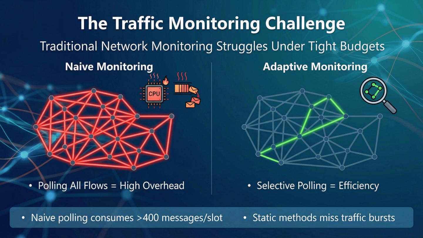 |
The fundamental challenge in modern SDN monitoring is a critical paradox: we need fine-grained traffic data, but the cost of comprehensive measurement is simply prohibitive. Network operators are constantly forced to balance three competing demands: they need accurate measurements for capacity planning, they must maintain low control-plane overhead, and they need a system that adapts instantly to changing network conditions. Current solutions fail this balance. They treat monitoring as a static problem, either polling everything constantly, which generates massive overhead, or using fixed heuristics that quickly become irrelevant when traffic patterns shift. This leaves operators blind to critical changes. We see that naive polling quickly becomes infeasible in large topologies, often consuming excessive control-plane bandwidth. We need a system that can make informed, adaptive decisions about what to measure, when to measure it, and where to measure from. This leads us to consider how existing research has attempted to solve this problem.
|
| ICACT20260358 Slide.03
[Big Slide]
[YouTube] |
Chrome Click!! |
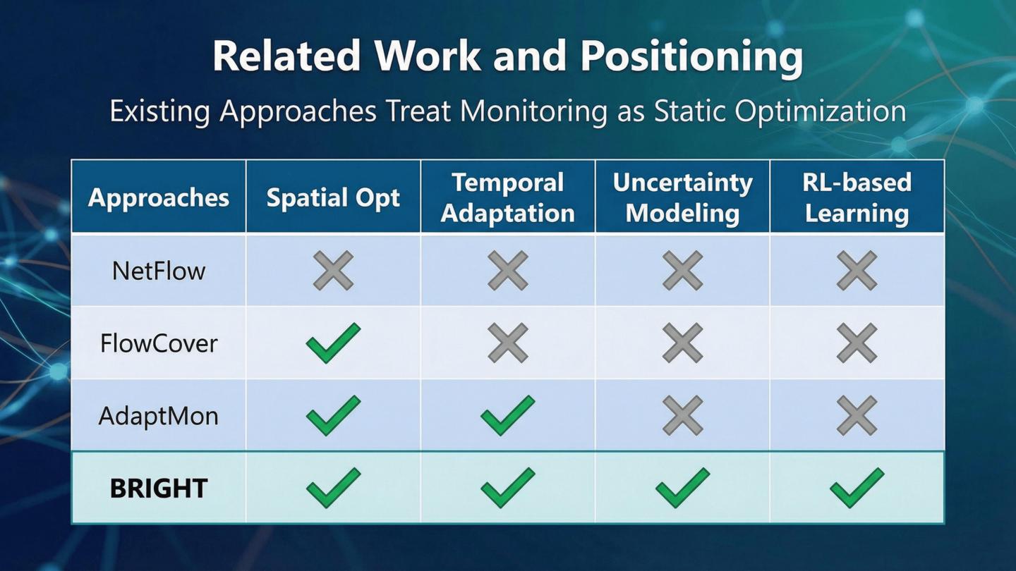 |
Before diving into BRIGHT, its important to position our work relative to the existing landscape. Previous research has largely focused on two areas: either optimizing the measurement process itself, or applying machine learning to traffic prediction. For instance, some work focuses on low-cost monitoring techniques, but these often lack the adaptability needed for dynamic environments. Other adaptive methods exist, but they typically rely on fixed heuristics or simple rate-based thresholds, meaning they cant effectively quantify or manage measurement uncertainty. Our key contribution is bridging this gap. We are the first to integrate Bayesian state estimation—which explicitly models uncertainty—with a reinforcement learning policy for dynamic resource allocation. This unified approach allows BRIGHT to continuously learn the optimal monitoring strategy based on the current network state and the inherent uncertainty of our estimates. This integration is what sets BRIGHT apart and allows us to model monitoring as a sequential decision process.
|
| ICACT20260358 Slide.04
[Big Slide]
[YouTube] |
Chrome Click!! |
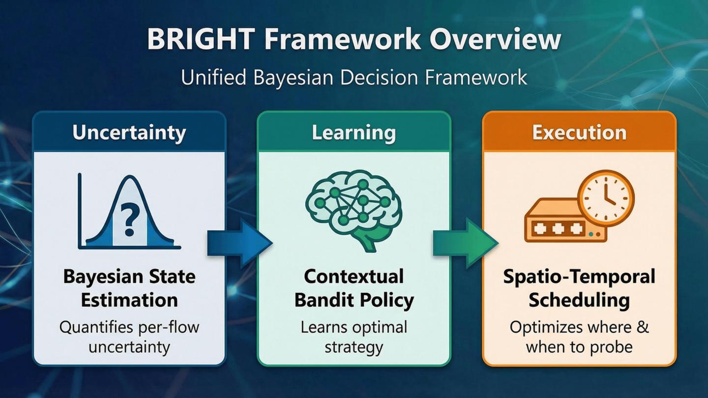 |
BRIGHT solves the limitations of static monitoring by modeling it as a sequential decision process that continuously learns and adapts. Our framework is built on the novel integration of three core technologies. First, we use Bayesian state estimation to maintain a lightweight Gaussian posterior for every active flow. This is crucial because it allows us to quantify uncertainty, distinguishing between flows we know well and flows that require more attention. Second, we employ a contextual bandit approach for policy learning. This system automatically selects the optimal monitoring template—a strategy that specifies the total budget and which flows to prioritize—based on the current network state. Finally, a spatio-temporal scheduler maps that selected template into concrete probing decisions, minimizing the cost of each query and balancing the load across switches. This three-part architecture ensures that BRIGHT is both uncertainty-aware and highly adaptive, allowing us to focus our limited resources where they matter most. Now, lets look at the mathematical foundation that underpins this framework.
|
| ICACT20260358 Slide.05
[Big Slide]
[YouTube] |
Chrome Click!! |
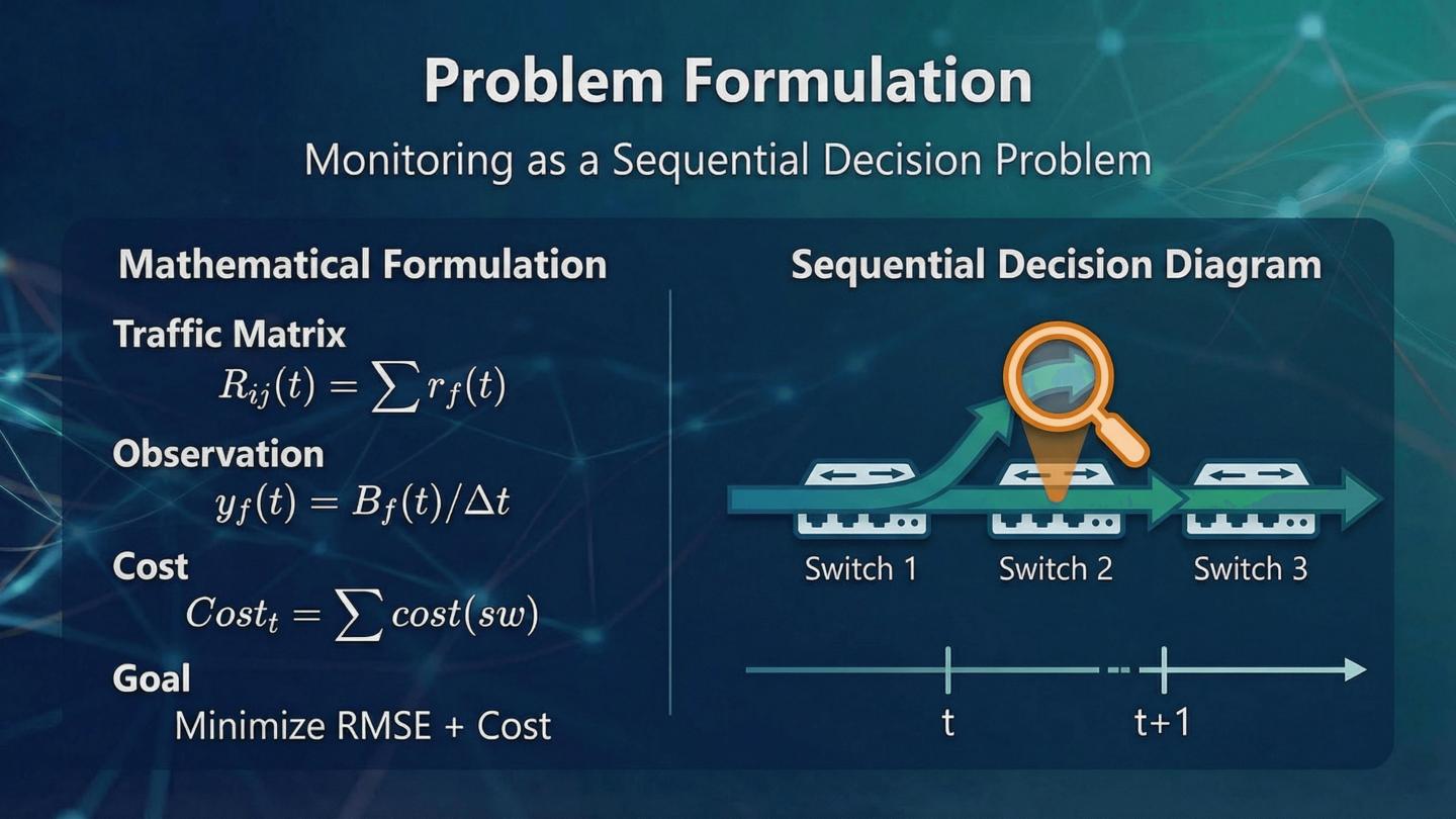 |
To formalize the problem, we model traffic monitoring as a sequential decision-making process under uncertainty. Our goal is to minimize the combined cost of measurement error and monitoring overhead over time. This is a complex optimization problem because the state of the network—the true traffic matrix—is only partially observable. We define the state of the system by the current traffic matrix and the accumulated uncertainty in our flow estimates. The action space is the selection of a monitoring template, which dictates the probing intensity. The reward function is designed to balance three competing objectives: maximizing accuracy, minimizing control-plane overhead, and ensuring fair load balancing across switches. Specifically, the reward is the negative sum of the traffic matrix RMSE, the monitoring cost, and the variance in switch load. By framing the problem this way, we can apply the powerful tools of reinforcement learning to find the optimal policy. This mathematical framework allows BRIGHT to learn the trade-offs between accuracy and efficiency automatically. Next, well examine the detailed architecture that implements this formulation.
|
| ICACT20260358 Slide.06
[Big Slide]
[YouTube] |
Chrome Click!! |
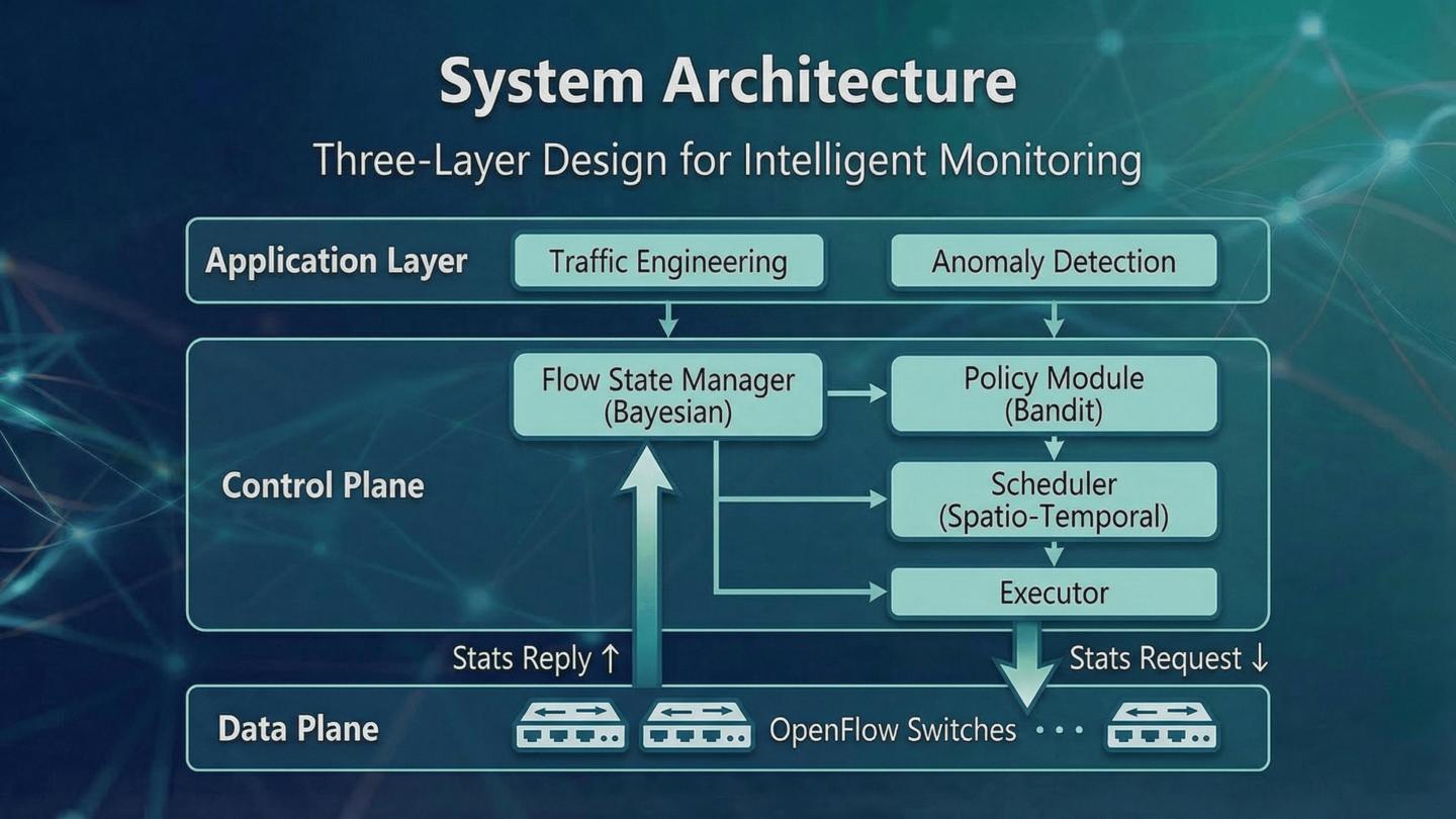 |
Lets look at how we architected BRIGHT to function within a standard SDN environment. We designed BRIGHT as a three-layer system to cleanly separate the core intelligence from the physical data plane. The Application Layer sits at the top, consuming our accurate traffic matrices for things like traffic engineering and anomaly detection. This is the business logic that drives the whole monitoring process. The real intelligence lives in the Control Plane. Here, five key modules work together to execute the adaptive monitoring loop. The Flow State Manager is critical; it holds the Bayesian model for every flow, giving us the estimate and the uncertainty. The Policy Module, which well discuss shortly, decides the overall monitoring strategy by selecting a template. Then, the Spatio-temporal Scheduler translates that high-level strategy into concrete OpenFlow requests, deciding exactly which switch to query and when. Finally, the Data Plane is just the standard OpenFlow switches, receiving requests and sending back counter samples. This modular design ensures that BRIGHT is both powerful and compatible with existing SDN infrastructure. This leads us directly to the foundation of our intelligence: the Bayesian state estimation.
|
| ICACT20260358 Slide.07
[Big Slide]
[YouTube] |
Chrome Click!! |
 |
Lets look at the core mechanism that allows BRIGHT to be uncertainty-aware: the Bayesian flow state estimation. For every active flow in the network, we dont just track a single rate estimate; we maintain a full Gaussian posterior distribution. This distribution, represented by the mean mu and the variance sigma squared, captures both our best guess of the flow rate and how confident we are in that guess. When we receive a new counter sample from a switch, we use standard Bayesian inference to update this posterior. The key here is that the new measurement is combined with our prior belief, giving us a refined estimate. If the new measurement is close to our prior mean, the variance shrinks significantly, meaning our confidence goes up. If the measurement is surprising, the mean shifts, but the variance might not shrink as much. This process is lightweight and runs continuously for thousands of flows, giving us a real-time, principled measure of estimation quality. But just knowing the posterior isnt enough; we need to turn that into actionable intelligence, which requires quantifying the uncertainty.
|
| ICACT20260358 Slide.08
[Big Slide]
[YouTube] |
Chrome Click!! |
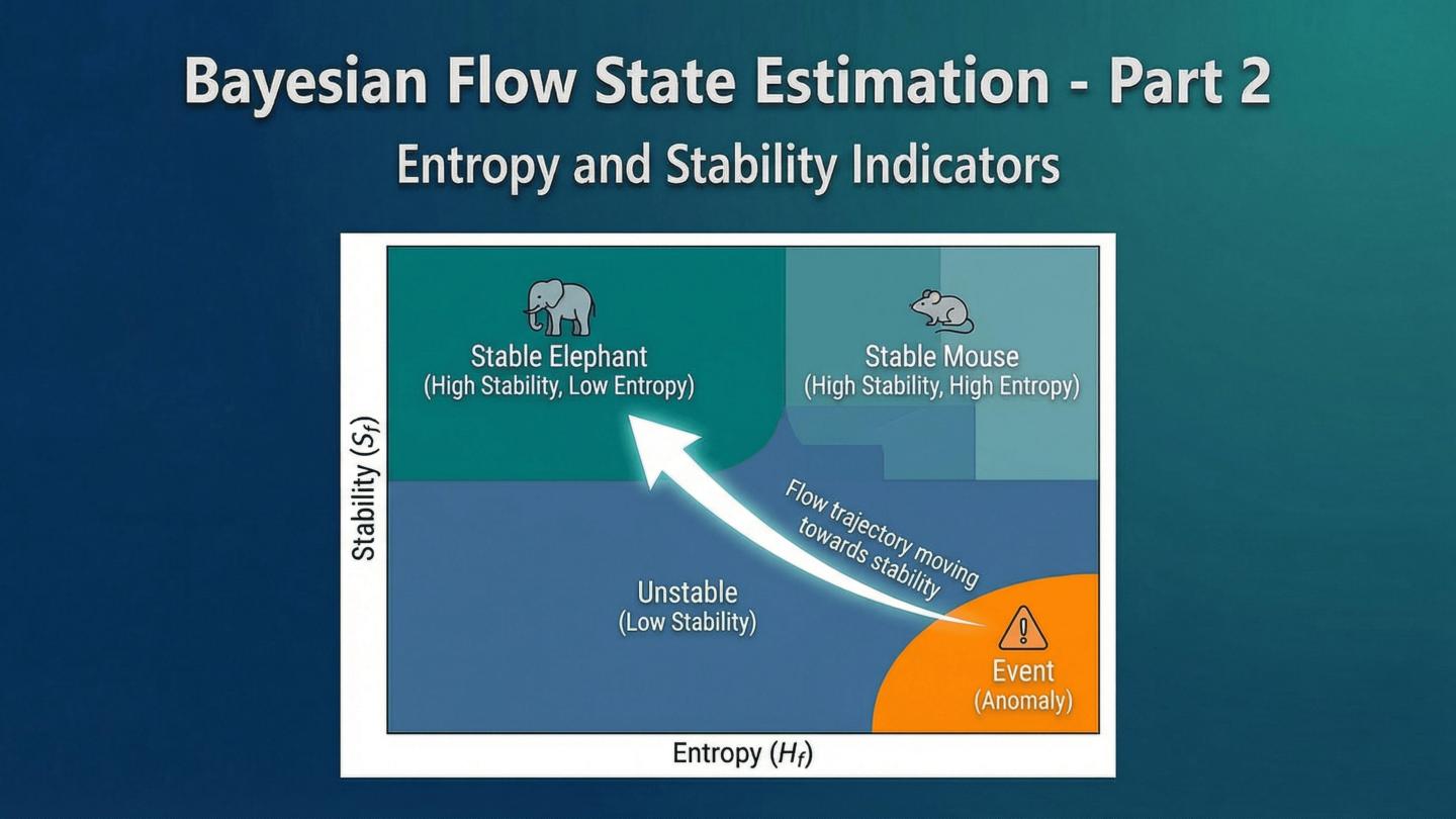 |
Lets look at how we translate the Bayesian posterior into concrete metrics that drive our monitoring decisions. From the Gaussian posterior, we derive two crucial uncertainty indicators: differential entropy and stability score. The differential entropy, H sub f, is a direct measure of how spread out our posterior distribution is. Higher entropy means greater uncertainty in the flow rate estimate, signaling that we need to probe that flow more frequently. This is a fundamental, information-theoretic measure of uncertainty. The second metric is the stability score, S sub f. This score quantifies the volatility of the flow rate itself, based on the sample variance of recent observations. A flow with a high stability score is highly unstable, meaning its rate is fluctuating rapidly. This is important because even if we have a low-entropy estimate right now, a highly unstable flow is likely to change soon. Using these two indicators, we automatically classify flows into four categories: stable elephants, stable mice, unstable flows, and event flows. This uncertainty-aware classification is the key to BRIGHTs efficiency, allowing us to concentrate our limited monitoring budget exactly where its needed most. This classification then feeds directly into our policy learning framework.
|
| ICACT20260358 Slide.09
[Big Slide]
[YouTube] |
Chrome Click!! |
 |
"Lets look at the policy framework that decides the overall monitoring strategy. We model the monitoring decision as a contextual bandit problem. This is far more flexible than using fixed heuristics because it allows the system to learn the optimal strategy through continuous interaction. The core idea is that we selected from a finite set of monitoring templates, or arms, each representing a different strategy—for example, an aggressive template that probes frequently versus a conservative one. At every decision epoch, BRIGHT constructs a context vector that captures the current network state. This context includes things like the recent traffic-matrix error, the average flow uncertainty we just discussed, and the current monitoring cost. Given this context, the policy module uses Thompson sampling to select the template that is predicted to yield the highest reward. This approach naturally balances exploration—trying out new templates—with exploitation—sticking to the best-performing template. The system learns a linear mapping from the network context to the expected reward for each template, ensuring that our monitoring strategy adapts dynamically to changing network conditions. But for this learning to work, we need a well-designed reward signal." |
| ICACT20260358 Slide.10
[Big Slide]
[YouTube] |
Chrome Click!! |
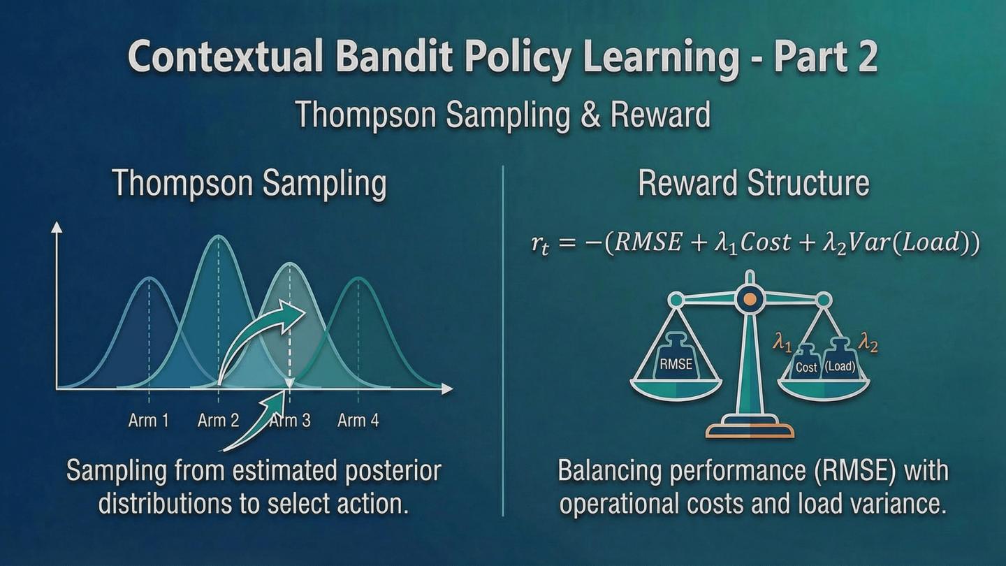 |
Lets look at how we design the reward signal to guide the contextual bandit policy. The reward function is the most critical part of any reinforcement learning system because it defines what "optimal" means. For BRIGHT, optimal monitoring must balance three competing objectives: accuracy, efficiency, and load balancing. Our reward function is designed to maximize accuracy while minimizing cost and congestion. We penalize the system based on three components. First, the RMSE, or the root mean square error, of the traffic matrix estimate. We want this to be low. Second, the monitoring cost, which is the total number of OpenFlow messages sent. We want this to be low for efficiency. And third, the variance of the monitoring load across all switches. We want this to be low to prevent any single switch from becoming a bottleneck. By combining these three terms into a single negative reward, the policy is forced to find a sweet spot: a strategy that is accurate enough, but also highly efficient and fair in its resource usage. This multi-objective reward design is what allows BRIGHT to achieve high performance without causing control-plane congestion. Now that weve selected a template, we need to execute it using our spatio-temporal scheduler.
|
| ICACT20260358 Slide.11
[Big Slide]
[YouTube] |
Chrome Click!! |
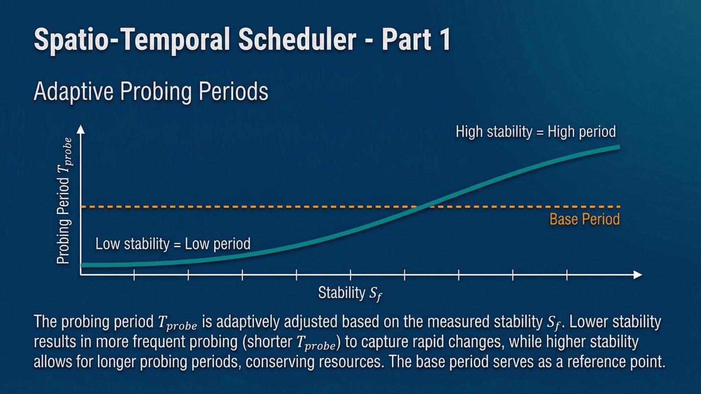 |
Lets look at how BRIGHT translates the policy decision into an actual probing schedule. Weve established that the contextual bandit selects a monitoring template, but that template only specifies a budget and base probing periods. The Spatio-Temporal Scheduler is responsible for the fine-grained allocation of those resources. This first part focuses on the temporal dimension: determining *when* to probe each flow. The core idea here is to dynamically adjust the probing period based on the flows stability. We start with the base probing period T_base, which is defined by the selected template and the flows category—remember, we classify flows into stable elephant, stable mouse, unstable, and event flows. We then use a proportional controller to adjust this period based on the flows stability score, S_f. If a flow is highly unstable, meaning its rate is fluctuating significantly, its stability score is low. This drives the probing period T_probe,f down, meaning we probe it more frequently. Conversely, a very stable flow gets a longer probing period, reducing overhead. This adaptive mechanism ensures that our limited monitoring budget is concentrated on the flows that are most difficult to estimate accurately, directly addressing the uncertainty quantified by the Bayesian model. This intelligent temporal allocation is critical for maximizing the accuracy we get from every single probe. Now we move to the second part of the scheduler: the spatial dimension.
|
| ICACT20260358 Slide.12
[Big Slide]
[YouTube] |
Chrome Click!! |
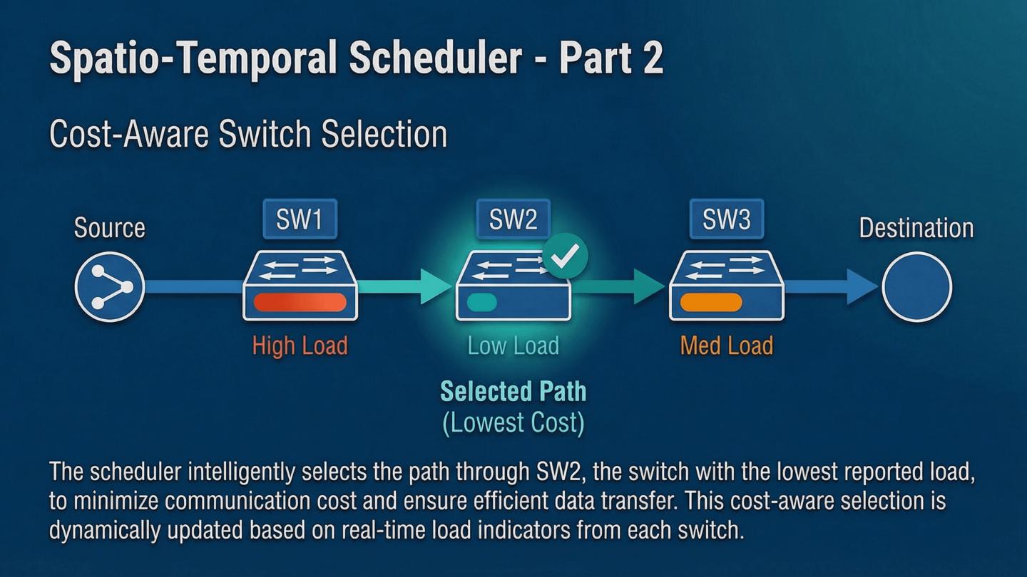 |
Having determined *when* to probe each flow, we now address the spatial dimension: *where* to probe it. This is a crucial optimization because polling different switches along a flows path incurs different costs and contributes differently to the overall load balancing. For every flow that needs to be probed in a given time slot, BRIGHT doesnt just pick the first switch. Instead, we consider all candidate switches along that flows path. We then select the switch that minimizes the total cost function. This cost function is designed to achieve two goals simultaneously: first, it minimizes the immediate cost of the query, and second, it ensures load balancing across all switches. By dynamically selecting the lowest-cost switch for each probe, we prevent any single switch from becoming a bottleneck due to excessive monitoring requests. This two-stage spatio-temporal approach—adjusting the probing frequency based on flow stability and selecting the polling switch based on cost and load—allows BRIGHT to achieve a fine-grained, highly efficient allocation of monitoring resources. This joint optimization is what truly sets our scheduler apart. With the scheduler detailed, lets put all these components together and see the main loop of the BRIGHT algorithm.
|
| ICACT20260358 Slide.13
[Big Slide]
[YouTube] |
Chrome Click!! |
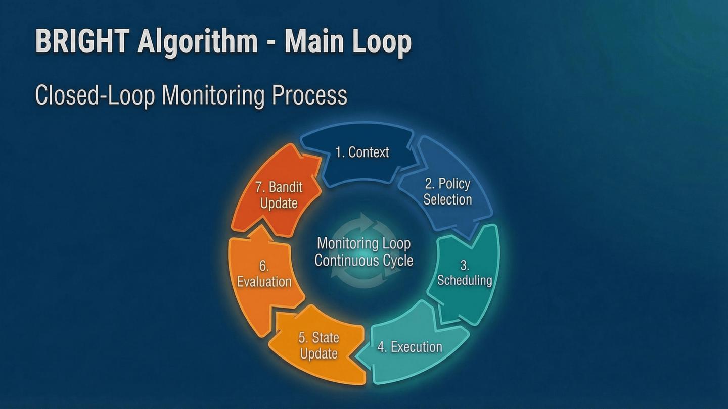 |
Weve now covered the three core components of BRIGHT: the Bayesian state estimation, the contextual bandit policy, and the spatio-temporal scheduler. This slide shows how they all fit together in the main operational loop. The process is continuous and slot-based. At the start of every time slot, the system first updates the flow state and uncertainty using any new counter samples collected in the previous slot. This is where the Bayesian model refines its estimates. Next, the Policy Module takes the current network state—the context—and uses the learned contextual bandit policy to select the optimal monitoring template for the next slot. This template dictates the overall monitoring intensity. Once the template is selected, the Spatio-Temporal Scheduler kicks in. It first determines the probing period for every flow based on its stability and the templates base period. Then, it selects the lowest-cost switch for each flow that needs to be probed in this slot. Finally, the Probe Executor sends the OpenFlow statistics requests to the selected switches, and the loop repeats. This continuous cycle of observe, decide, and act is the essence of BRIGHT. It ensures that monitoring is always adaptive, driven by uncertainty, and optimized for cost. This entire intelligence layer is implemented on the SDN controller, so lets look at the system implementation details.
|
| ICACT20260358 Slide.14
[Big Slide]
[YouTube] |
Chrome Click!! |
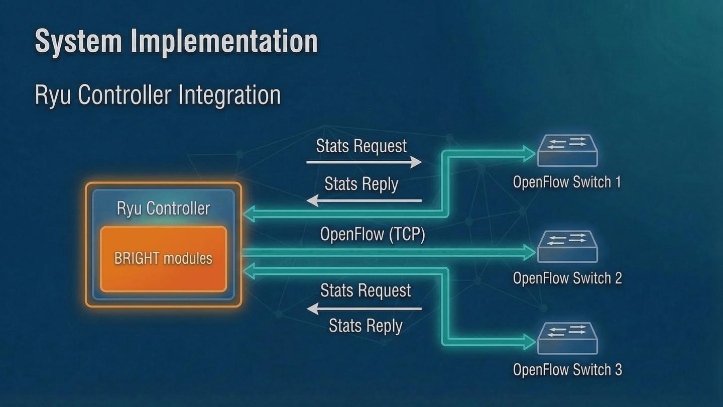 |
To demonstrate the practical feasibility of BRIGHT, we implemented the entire system on top of the Ryu SDN controller. This slide illustrates how our core modules integrate into a standard OpenFlow environment. The BRIGHT intelligence layer sits within the controller, communicating directly with the data plane—the OpenFlow switches—via the standard OpenFlow protocol. The Flow State and Uncertainty Manager, the Policy Module, and the Spatio-Temporal Scheduler all run as applications within the Ryu framework. The Probe Executor is responsible for sending the OpenFlow statistics requests, which are essentially the monitoring probes, and receiving the counter samples back from the switches. This design ensures that BRIGHT is fully compatible with existing SDN infrastructure. We didnt require any modifications to the OpenFlow protocol or the switch hardware itself. This modular, layered approach allows us to maintain the complex decision-making logic in the control plane while leveraging the high-performance measurement capabilities of the data plane. Now that weve covered the implementation, we can move on to the experimental setup and the metrics we used to evaluate BRIGHTs performance.
|
| ICACT20260358 Slide.15
[Big Slide]
[YouTube] |
Chrome Click!! |
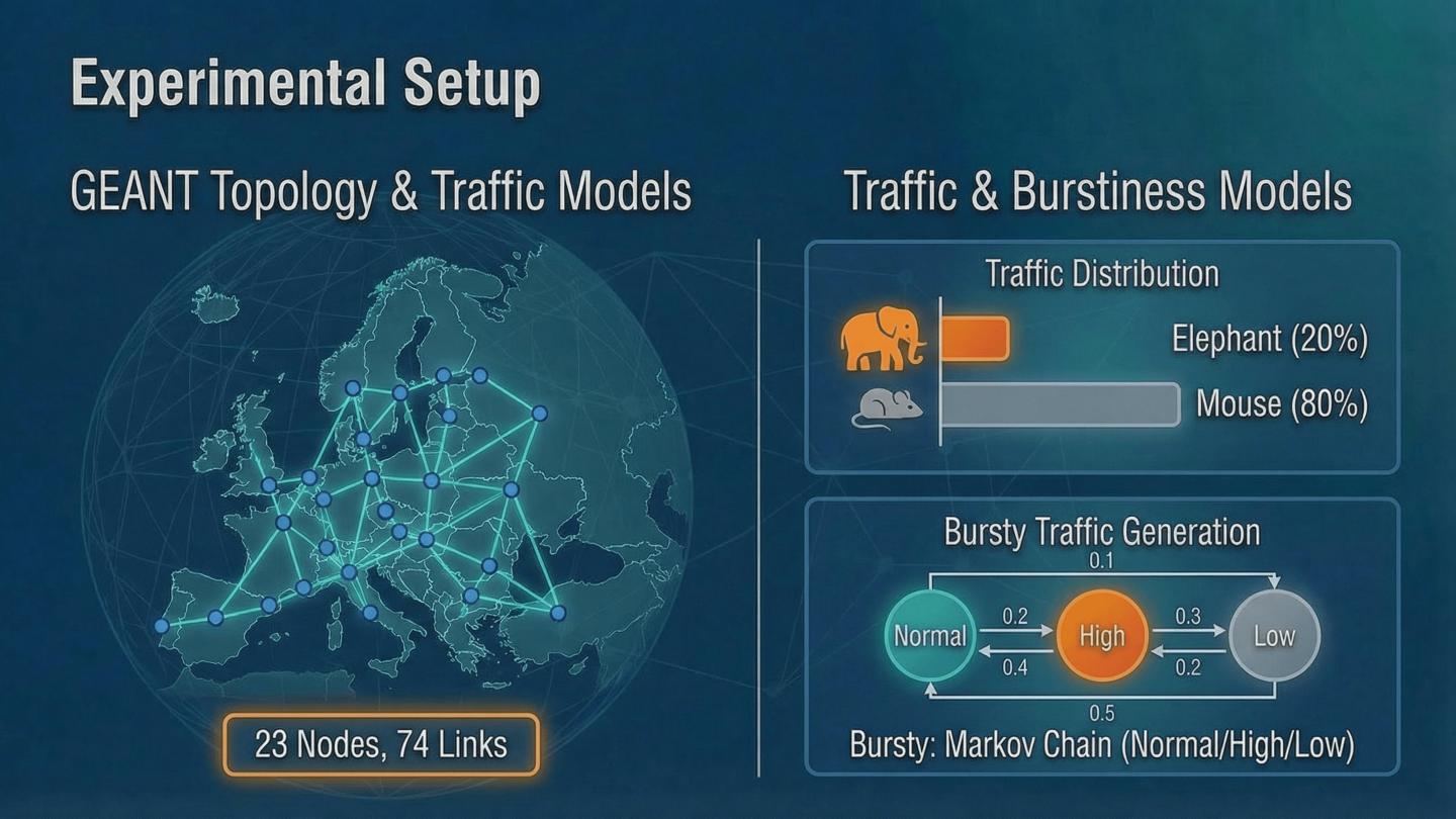 |
To rigorously evaluate BRIGHT, we established a comprehensive experimental setup and defined clear evaluation metrics. We used the well-known GEANT backbone topology, which consists of 23 nodes and 74 links, simulating a realistic wide-area network environment. Our traffic model included 100 active flows, categorized into elephant and mouse flows, with both stationary and bursty traffic scenarios to test adaptability. We compare BRIGHT against three state-of-the-art baselines: LCM, AdaptMon, and OpenTM, ensuring a fair comparison against existing adaptive and low-cost monitoring solutions. Our evaluation focuses on four key metrics. First, we measure the monitoring overhead, specifically the number of OpenFlow messages per slot, as this directly impacts control-plane capacity. Second, we look at the effective link utilization, which quantifies how much link capacity is preserved for actual data traffic versus monitoring traffic. Third, we track the control-plane latency, which indicates the controllers responsiveness under load. Finally, and most importantly, we measure the accuracy of the estimated traffic matrix using the Root Mean Square Error, or RMSE. This ensures that our efficiency gains do not compromise the quality of the measurement data. This setup allows us to demonstrate that BRIGHT provides superior efficiency and adaptability without sacrificing accuracy. Lets look at the results under stationary traffic conditions.
|
| ICACT20260358 Slide.16
[Big Slide]
[YouTube] |
Chrome Click!! |
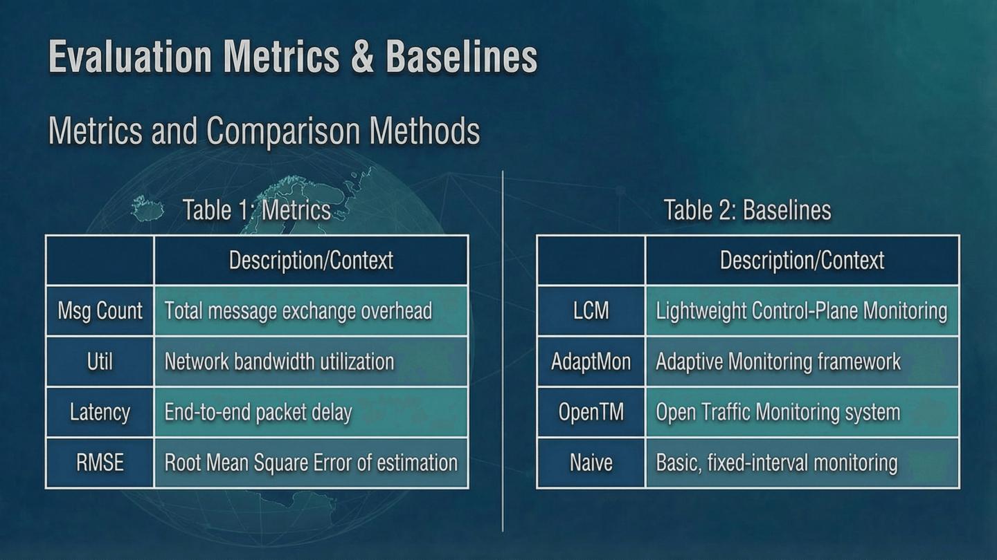 |
Lets look at the metrics we used to evaluate BRIGHT and the baselines we compared against. Our evaluation focuses on the critical trade-off between measurement accuracy and monitoring overhead. We used five primary metrics to capture this balance. First, we measured the total number of monitoring messages per slot, which directly quantifies the control-plane overhead. Minimizing this is crucial for controller stability. Second, we tracked the peak monitoring utilization, which tells us the maximum percentage of control-plane capacity consumed by monitoring tasks. Third, we looked at Effective Link Utilization, or EffUtil, which measures the fraction of link capacity available for actual data traffic after accounting for monitoring traffic. This is a key measure of efficiency. Fourth, we assessed the accuracy of the estimated traffic matrix using Root Mean Square Error, or RMSE. We must ensure that reducing overhead does not compromise the quality of the measurement data. Finally, we measured the control-plane latency to ensure our adaptive strategy does not introduce unacceptable delays. We compared BRIGHT against three state-of-the-art baselines: LCM, which focuses on low cost; AdaptMon, which uses adaptive sampling; and OpenTM, a standard OpenFlow traffic matrix estimator. These baselines represent the current spectrum of monitoring strategies. This comprehensive set of metrics allows us to rigorously demonstrate BRIGHTs superiority in both efficiency and accuracy. Now, lets examine the results under stationary traffic conditions.
|
| ICACT20260358 Slide.17
[Big Slide]
[YouTube] |
Chrome Click!! |
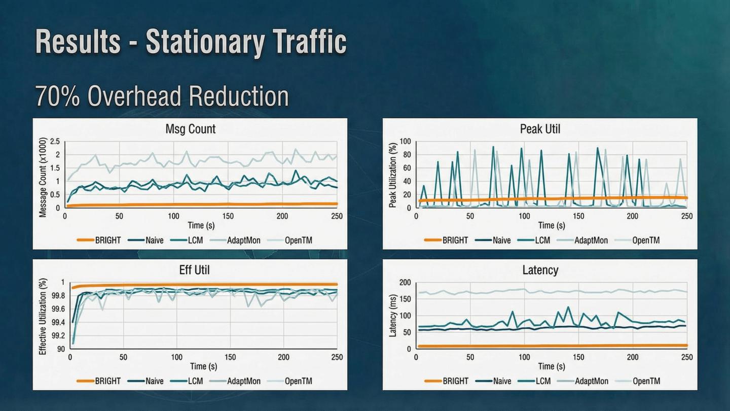 |
Lets look at the experimental results under stationary traffic conditions. The key takeaway here is that BRIGHT drastically reduces monitoring overhead without sacrificing accuracy. We see that BRIGHT consistently achieves the lowest number of monitoring messages per slot, hovering around 100 messages. This represents a 50 to 70 percent reduction compared to the baselines, which require between 200 and 350 messages. This efficiency gain is directly attributable to our Bayesian uncertainty modeling and the contextual bandit policy, which intelligently selects only the most necessary probes. Furthermore, BRIGHT maintains the highest Effective Link Utilization, near 99.6 percent. This means more network capacity is dedicated to user data rather than measurement overhead. This is a significant gain in large-scale networks. Importantly, our traffic matrix accuracy, measured by RMSE, remains competitive with the baselines. We prove that we can be highly efficient while still providing high-quality measurement data. The control-plane latency is also the lowest and most stable for BRIGHT, indicating that the controller is not being overwhelmed by monitoring requests. These results confirm BRIGHTs ability to operate efficiently in stable environments. But what happens when the network becomes dynamic? Lets look at the bursty traffic results. |
| ICACT20260358 Slide.18
[Big Slide]
[YouTube] |
Chrome Click!! |
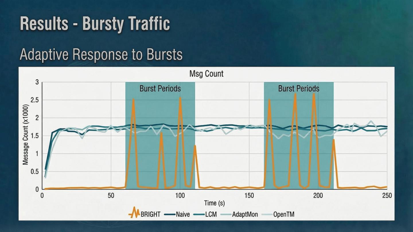 |
Lets look at how BRIGHT performs under bursty traffic, which is a much more challenging scenario. We introduced random traffic bursts to 30 percent of the flows, simulating real-world network dynamics. The core challenge is adapting quickly to these bursts without over-provisioning the monitoring system. The results show BRIGHTs superior adaptability. During burst intervals, BRIGHT correctly identifies the increased uncertainty and moderately increases its probing rate. However, even during these peaks, our monitoring message count remains significantly lower than all baselines. This demonstrates that the contextual bandit policy is successfully learning to increase measurement intensity only when and where it is needed. Crucially, BRIGHT quickly returns to a low overhead state once the burst subsides, unlike the baselines which tend to maintain persistently high probing rates. This adaptive behavior is key to long-term efficiency. We also observe that BRIGHT maintains the highest Effective Link Utilization throughout the experiment, even during the bursts. This means our system preserves data traffic capacity when the network is under stress. Finally, BRIGHT exhibits the smallest and most stable control-plane latency, preventing controller congestion even when the traffic is highly dynamic. These results validate the power of integrating Bayesian uncertainty with reinforcement learning for dynamic resource allocation. This leads us to the key insights derived from our design and evaluation. |
| ICACT20260358 Slide.19
[Big Slide]
[YouTube] |
Chrome Click!! |
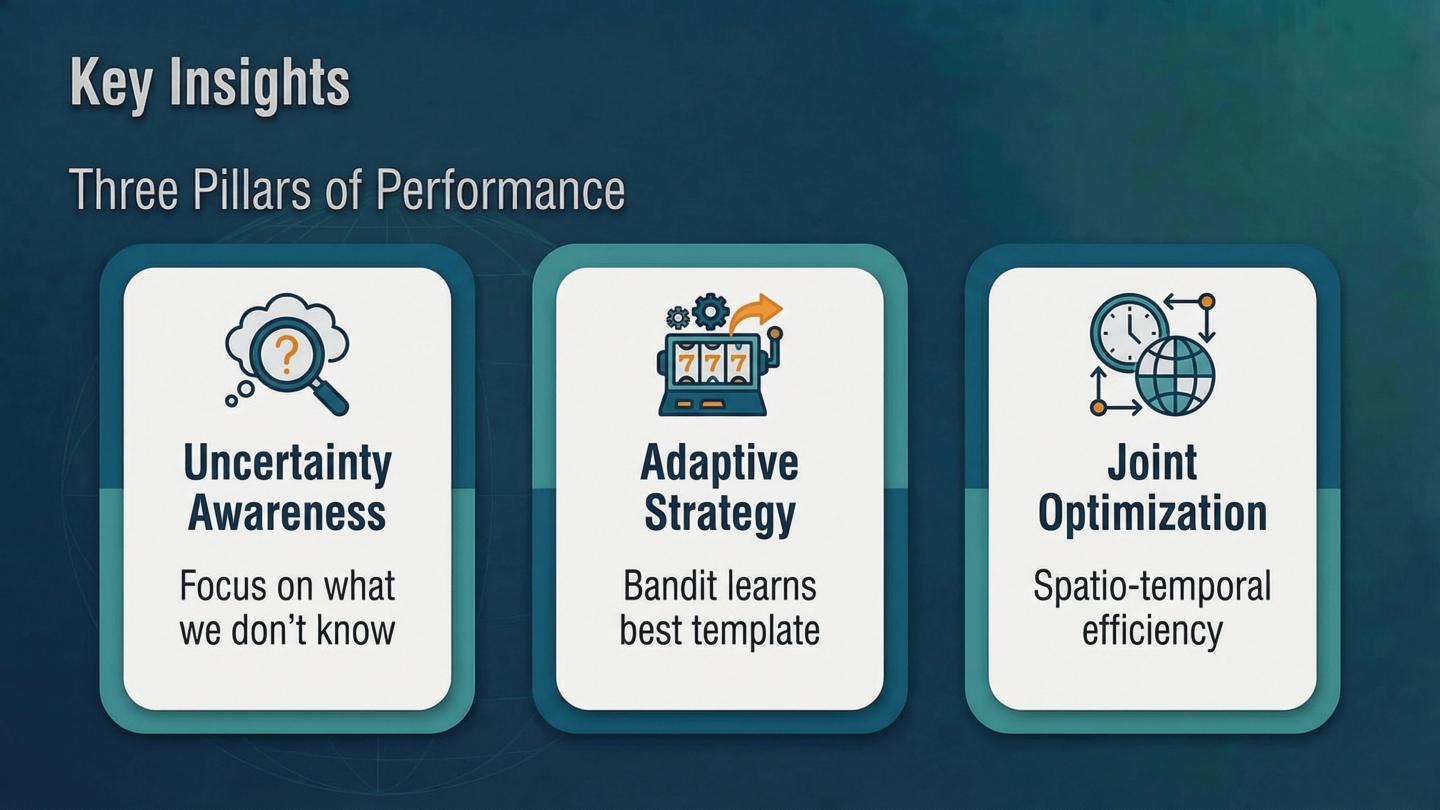 |
Lets look at the key insights that drove the design of BRIGHT and explain why our approach is so effective. The fundamental insight is that network monitoring should be treated as a sequential decision problem under uncertainty, not a static optimization. This led us to three core design choices. First, the Bayesian Flow State Estimation is critical because it provides a principled way to quantify uncertainty. By modeling the variance of a flows rate, we can prioritize monitoring resources on flows that are difficult to estimate, rather than just the largest flows. This is a fundamental shift from rate-based heuristics. Second, the Contextual Bandit Policy Learning allows the system to automatically learn the optimal monitoring strategy. We dont rely on manual tuning of parameters. The system learns which template—aggressive or conservative—works best given the current network state and its associated cost and accuracy trade-offs. This provides the necessary adaptability. Third, the Spatio-Temporal Probing Scheduler ensures that the selected monitoring budget is executed with maximum efficiency. By jointly optimizing when to probe a flow and which switch along its path to query, we minimize the total control-plane cost and balance the load across the network. These three components work in concert to achieve the high efficiency and accuracy we observed in the experiments. Now, lets summarize the overall impact of this work. |
| ICACT20260358 Slide.20
[Big Slide]
[YouTube] |
Chrome Click!! |
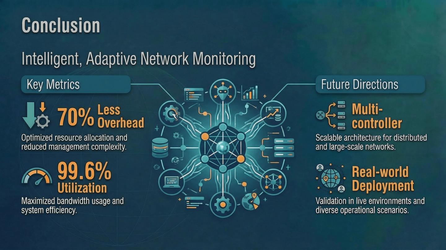 |
Lets look at the conclusion and the overall impact of the BRIGHT framework. We have demonstrated that integrating Bayesian uncertainty modeling with reinforcement learning creates a powerful, adaptive solution for network monitoring. BRIGHT moves beyond static optimization by continuously learning and adapting its measurement strategy to the current network state. The experimental results confirm significant practical benefits. BRIGHT reduces monitoring overhead by 50 to 70 percent compared to state-of-the-art methods, which frees up critical control-plane resources. This efficiency gain translates directly into improved effective link utilization, ensuring more network capacity is available for user data. Crucially, we achieve this efficiency while maintaining or even improving traffic-matrix estimation accuracy. BRIGHTs ability to adapt intelligently to bursty traffic is perhaps its most important feature, ensuring stable performance even under dynamic conditions. These improvements mean network operators can deploy fine-grained monitoring in large-scale SDN environments without incurring prohibitive costs or manual tuning. Looking ahead, we plan to extend BRIGHT to multi-controller deployments for greater scalability and integrate it with other SDN applications like routing and resource allocation. Thank you for your time. I am now happy to take any questions. |
| |